Experimental results
bayesian model outputs
Oocyte diameter
Code
#| class-source: fold-hide
#| message: false
#| warning: false
#| fig-width: 9.5
#| fig-height: 5

library(tidyverse)
library(janitor)
library(readxl)
library(brms)
library(patchwork)
library(reefspawn)

egg_diameter_output <- readxl::read_excel("/Users/rof011/reefspawn/code/SurvExpData.xlsx", sheet = "ReprodOutput") |>
  janitor::clean_names() |>
  dplyr::rename(
    area = colony_size_cm2,
    egg_cover = egg_percent_cover_jar,
    egg_depth = egg_layer_tickness_mm,
    egg_diameter = mean_egg_diameter_um
  ) |>
  dplyr::mutate(
    egg_diameter = as.numeric(egg_diameter),
    treatment = dplyr::case_when(
      stringr::str_detect(treatment, "SURV") ~ "impacted",
      stringr::str_detect(treatment, "NORM") ~ "unimpacted",
      TRUE ~ NA_character_
    )
  ) |>
  dplyr::select(treatment, species, egg_diameter) |>
  tidyr::drop_na() |>
  dplyr::mutate(var = paste0(species, "_", treatment))

# Fit model including species
# fm_egg_size <- brms::brm(
#   egg_diameter ~ treatment * species,
#   data = egg_diameter_output,
#   cores = 10,
#   chains = 4,
#   iter = 6000
# )
#
# saveRDS(fm_egg_size, "/Users/rof011/reefspawn/code/fm_egg_size.rds")

fm_egg_size <- readRDS("/Users/rof011/reefspawn/code/fm_egg_size.rds")

# Fitted posterior summaries
fitted_vals <- fitted(fm_egg_size, scale = "response")
egg_diameter_output <- egg_diameter_output |>
  mutate(
    predicted = fitted_vals[, "Estimate"],
    lower = fitted_vals[, "Q2.5"],
    upper = fitted_vals[, "Q97.5"]
  )

# Summarise for model overlay
egg_diameter_summary <- egg_diameter_output |>
  group_by(species, treatment) |>
  summarise(
    predicted = unique(predicted),
    lower = unique(lower),
    upper = unique(upper),
    .groups = "drop"
  )

# Plot
a <- ggplot() +
  theme_bw() +
  facet_wrap(~ species) +
  geom_violin(
    data = egg_diameter_output,
    aes(x = treatment, y = egg_diameter, fill = treatment),
    color = "grey50", scale = "width", alpha = 0.6, show.legend = FALSE
  ) +
  geom_jitter(
    data = egg_diameter_output,
    aes(x = treatment, y = egg_diameter, fill = treatment),
    width = 0.05, alpha = 0.5, show.legend = FALSE
  ) +
  geom_boxplot(
    data = egg_diameter_summary,
    aes(x = treatment, fill = treatment,
        lower = lower, upper = upper,
        middle = predicted, ymin = lower, ymax = upper),
    stat = "identity", width = 0.2, alpha = 0.4, show.legend = FALSE
  ) +
  labs(y = "Egg size (µm)", title = "Egg size by Treatment") +
  scale_fill_manual(values = c("navajowhite2", "paleturquoise")) +
  scale_y_continuous(limits = c(0, 1000))

a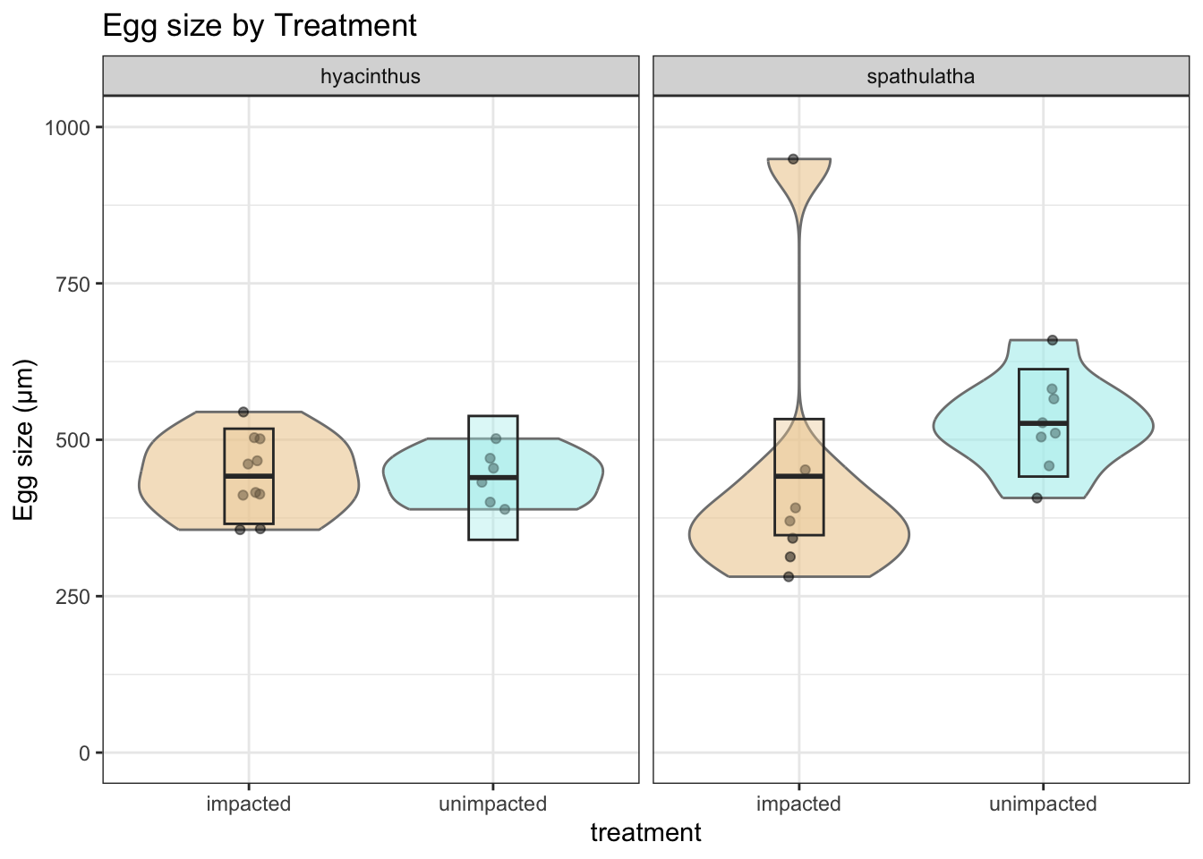
Code
colony_area_output <- readxl::read_excel("/Users/rof011/reefspawn/code/SurvExpData.xlsx", sheet = "ReprodOutput") |>
  janitor::clean_names() |>
  dplyr::rename(
    area = colony_size_cm2,
    egg_cover = egg_percent_cover_jar,
    egg_depth = egg_layer_tickness_mm,
    egg_diameter = mean_egg_diameter_um
  )|>
  dplyr::select(treatment, species, area) |>
  tidyr::drop_na() |>
  dplyr::mutate(var = paste0(species, "_", treatment))

# check colony area differences

# fm_area <- brms::brm(
#   area ~  species,
#   data = colony_area_output,
#   cores = 10,
#   chains = 4,
#   iter = 6000
# )
#
# saveRDS(fm_area, "/Users/rof011/reefspawn/code/fm_area.rds")

fm_area <- readRDS("/Users/rof011/reefspawn/code/fm_area.rds")
Code
hypothesis(fm_egg_size, "treatmentunimpacted = 0")Hypothesis Tests for class b:
Hypothesis Estimate Est.Error CI.Lower CI.Upper Evid.Ratio
1 (treatmentunimpac... = 0 -2.23 65.03 -131.47 125.31 NA
Post.Prob Star
1 NA
---
'CI': 90%-CI for one-sided and 95%-CI for two-sided hypotheses.
'*': For one-sided hypotheses, the posterior probability exceeds 95%;
for two-sided hypotheses, the value tested against lies outside the 95%-CI.
Posterior probabilities of point hypotheses assume equal prior probabilities.No strong evidence of a treatment effect in hyacinthus.
Estimate –0.38 [–130.57, +128.79M]
Code
hypothesis(fm_area, "speciesspathulatha = 0")Hypothesis Tests for class b:
Hypothesis Estimate Est.Error CI.Lower CI.Upper Evid.Ratio
1 (speciesspathulatha) = 0 -600.54 121.09 -839.39 -359.22 NA
Post.Prob Star
1 NA *
---
'CI': 90%-CI for one-sided and 95%-CI for two-sided hypotheses.
'*': For one-sided hypotheses, the posterior probability exceeds 95%;
for two-sided hypotheses, the value tested against lies outside the 95%-CI.
Posterior probabilities of point hypotheses assume equal prior probabilities.No strong evidence of a difference in area between species.
Estimate –600.5 [–839.39, +359.22]
Code
hypothesis(fm_egg_size, "speciesspathulatha = 0")Hypothesis Tests for class b:
Hypothesis Estimate Est.Error CI.Lower CI.Upper Evid.Ratio
1 (speciesspathulatha) = 0 -0.16 61.19 -119.61 121.28 NA
Post.Prob Star
1 NA
---
'CI': 90%-CI for one-sided and 95%-CI for two-sided hypotheses.
'*': For one-sided hypotheses, the posterior probability exceeds 95%;
for two-sided hypotheses, the value tested against lies outside the 95%-CI.
Posterior probabilities of point hypotheses assume equal prior probabilities.Oocyte biomass
Code
#| class-source: fold-hide
#| message: false
#| warning: false
#| fig-width: 9.5
#| fig-height: 5

reproductive_output <- readxl::read_excel("/Users/rof011/reefspawn/code/SurvExpData.xlsx", sheet = "ReprodOutput") |>
  janitor::clean_names() |>
  dplyr::rename(area = colony_size_cm2) |>
  dplyr::mutate(
    egg_cover = as.numeric(egg_percent_cover_jar),
    egg_depth = as.numeric(egg_layer_tickness_mm),
    egg_diameter = as.numeric(mean_egg_diameter_um),
    treatment = dplyr::case_when(
      stringr::str_detect(treatment, "SURV") ~ "impacted",
      stringr::str_detect(treatment, "NORM") ~ "unimpacted",
      TRUE ~ NA_character_
    )
  ) |>
  dplyr::select(treatment, species, area, egg_diameter, egg_cover, egg_depth) |>
  dplyr::rowwise() |>
  dplyr::mutate(output = calculate_egg_densities(egg_diameter,egg_cover, egg_depth, method = "3d_packing"),
                output2 = calculate_egg_densities(egg_diameter,egg_cover, egg_depth, method = "layered")
    ) |>
  dplyr::ungroup() |>
  dplyr::mutate(var = paste0(species, "_", treatment)) |>
  tidyr::drop_na() |>
  mutate(output = output / area,
         output2 = output2 / area)

# # Fit model with species interaction
# fm_reproductive_output <- brm(
#   output ~ treatment * species,
#   data = reproductive_output,
#   cores = 10,
#   chains = 4,
#   iter = 6000
# )
#
# saveRDS(fm_reproductive_output, "/Users/rof011/reefspawn/code/fm_reproductive_output.rds")

fm_reproductive_output <- readRDS("/Users/rof011/reefspawn/code/fm_reproductive_output.rds")

# Extract fitted values
fitted_vals <- fitted(fm_reproductive_output, scale = "response")

reproductive_output <- reproductive_output |>
  mutate(
    predicted = fitted_vals[, "Estimate"],
    lower = fitted_vals[, "Q2.5"],
    upper = fitted_vals[, "Q97.5"]
  )

# Summarise predictions per treatment × species for plotting box layer

reproductive_summary <- reproductive_output |>
  group_by(species, treatment) |>
  summarise(
    predicted = unique(predicted),
    lower = unique(lower),
    upper = unique(upper),
    .groups = "drop"
  )

# Plot
b <- ggplot() +
  theme_bw() +
  facet_wrap(~ species) +
  geom_violin(
    data = reproductive_output,
    aes(x = treatment, y = output, fill = treatment),
    color = "grey50", scale = "width", alpha = 0.6, show.legend = FALSE
  ) +
  geom_jitter(
    data = reproductive_output,
    aes(x = treatment, y = output, fill = treatment),
    width = 0.05, alpha = 0.5, show.legend = FALSE
  ) +
  geom_boxplot(
    data = reproductive_summary,
    aes(x = treatment, fill = treatment,
        lower = lower, upper = upper,
        middle = predicted, ymin = lower, ymax = upper),
    stat = "identity", width = 0.2, alpha = 0.7, show.legend = FALSE
  ) +
  labs(y = "Reproductive output (n per cm2)", title = "Reproductive output by Treatment") +
  scale_fill_manual(values = c("navajowhite2", "paleturquoise"))

b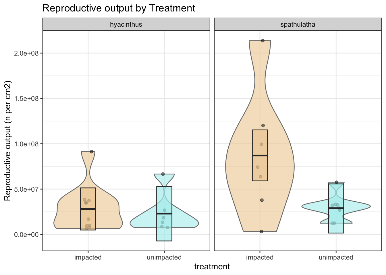
Code
hypothesis(fm_reproductive_output, "treatmentunimpacted = 0")Hypothesis Tests for class b:
Hypothesis Estimate Est.Error CI.Lower CI.Upper Evid.Ratio
1 (treatmentunimpac... = 0 -5138974 19355732 -42924849 32449033 NA
Post.Prob Star
1 NA
---
'CI': 90%-CI for one-sided and 95%-CI for two-sided hypotheses.
'*': For one-sided hypotheses, the posterior probability exceeds 95%;
for two-sided hypotheses, the value tested against lies outside the 95%-CI.
Posterior probabilities of point hypotheses assume equal prior probabilities.No strong evidence of a treatment effect in hyacinthus.
Estimate –5.5M [–43.8, +33.3]
Code
hypothesis(fm_reproductive_output, "treatmentunimpacted + treatmentunimpacted:speciesspathulatha = 0")Hypothesis Tests for class b:
Hypothesis Estimate Est.Error CI.Lower CI.Upper Evid.Ratio
1 (treatmentunimpac... = 0 -58137442 19952480 -97621677 -18695671 NA
Post.Prob Star
1 NA *
---
'CI': 90%-CI for one-sided and 95%-CI for two-sided hypotheses.
'*': For one-sided hypotheses, the posterior probability exceeds 95%;
for two-sided hypotheses, the value tested against lies outside the 95%-CI.
Posterior probabilities of point hypotheses assume equal prior probabilities.Strong evidence that reproductive output is lower in unimpacted spathulata
Estimate –57.9M [–96.7M, –18.9M]
Larval development
Code
#| class-source: fold-hide
#| message: false
#| warning: false
#| fig-width: 9.5
#| fig-height: 5


string_treatment <- c(rep("S1",3), rep("N2", 3), rep("S2", 3), rep("N1", 3))


onboard_cultures <- readxl::read_excel("/Users/rof011/reefspawn/code/SurvExpData.xlsx", sheet = "OnboardCulture") |>
  janitor::clean_names() |>
  # clean up time
  dplyr::mutate(time = as.POSIXct(samping_date, format = "%d/%m/%Y", tz = "UTC")) |>
  dplyr::mutate(time = as.numeric(difftime(time, min(time), units = "days"))) |>
  # clean up ID
  #dplyr::filter(!is.na(treatment_id)) |>
  dplyr::mutate(treatment = stringr::str_remove(treatment_id, "^Tank_")) |>
  dplyr::mutate(sample_prefix = ifelse(is.na(sample_id), NA, substr(sample_id, 1, 2))) |>
  dplyr::mutate(treatment = ifelse(is.na(treatment_id), sample_prefix, treatment_id)) %>%  # replace missing treatment_id with sample_prefix, check seperately
  dplyr::filter(treatment %in% c("N1", "N2", "S1", "S2")) %>%
  mutate(rep = rep(c("a", "b", "c"), (nrow(.)/3))) |>
  select(treatment, time, deformed, normal, total_larvae) |>
  group_by(treatment, time) |>
  summarise(deformed = mean(deformed), normal = mean(normal), total_larvae = mean(total_larvae)) |>
  dplyr::mutate(species = dplyr::case_when(
    stringr::str_detect(treatment, "1$") ~ "hyacinthus",
    stringr::str_detect(treatment, "2$") ~ "spathulata",
    TRUE ~ NA_character_
  )) |>
  dplyr::mutate(var = paste0(species, "_", treatment)) |>
  tidyr::separate(var, into = c("species", "treatment"), sep = "_") |>
  dplyr::mutate(condition = dplyr::case_when(
    stringr::str_detect(treatment, "^N") ~ "unimpacted",
    stringr::str_detect(treatment, "^S") ~ "impacted",
    TRUE ~ NA_character_
  )) |>
  mutate(total_larvae = (total_larvae/16) * 1000) |>
  mutate(treatment = condition)

# quadratic_counts <- brm(
#   total_larvae ~ time + I(time^2) * treatment * species,
#   data = onboard_cultures,
#   family = gaussian(),
#   chains = 4, cores = 4
# )

# saveRDS(quadratic_counts, "/Users/rof011/reefspawn/code/quadratic_counts.rds")

quadratic_counts <- readRDS("/Users/rof011/reefspawn/code/quadratic_counts.rds")


# Expand prediction grid with full interaction structure
newdata <- tidyr::expand_grid(
  time = seq(min(onboard_cultures$time), max(onboard_cultures$time), length.out = 100),
  treatment = unique(onboard_cultures$treatment),
  species = unique(onboard_cultures$species)
)

# Get predicted values with uncertainty
quad_fitted <- fitted(
  quadratic_counts,
  newdata = newdata,
  scale = "response",
  allow_new_levels = TRUE
) |> as_tibble()

# Combine predictions
newdata_quad <- bind_cols(newdata, quad_fitted)

# Add condition back (if needed for fill/color)
newdata_quad <- newdata_quad |>
  left_join(onboard_cultures |> distinct(treatment, species, condition), by = c("treatment", "species"))

# Plot
plot_c <- ggplot() +
  theme_bw() +
  facet_wrap(~ species) +
  geom_ribbon(data = newdata_quad, aes(x = time, ymin = Q2.5, ymax = Q97.5, fill = condition),
              alpha = 0.5, show.legend = FALSE) +
  geom_line(data = newdata_quad, aes(x = time, y = Estimate, color = condition),
            linewidth = 1.2, show.legend = FALSE) +
  geom_line(data = onboard_cultures, aes(x = time, y = total_larvae, color = condition),
            linetype = "dashed", show.legend = FALSE) +
  geom_point(data = onboard_cultures, aes(x = time, y = total_larvae, fill = condition),
             shape = 21, color = "black", size = 2, alpha = 0.9, show.legend = FALSE) +
  labs(
    title = "Quadratic fit of larval counts over time",
    y = "n larvae / litre",
    x = "Time (days)"
  ) +
  scale_fill_manual(values = c("navajowhite", "paleturquoise")) +
  scale_color_manual(values = c("navajowhite3", "paleturquoise3")) +
  coord_cartesian(ylim = c(0, 2500))


plot_c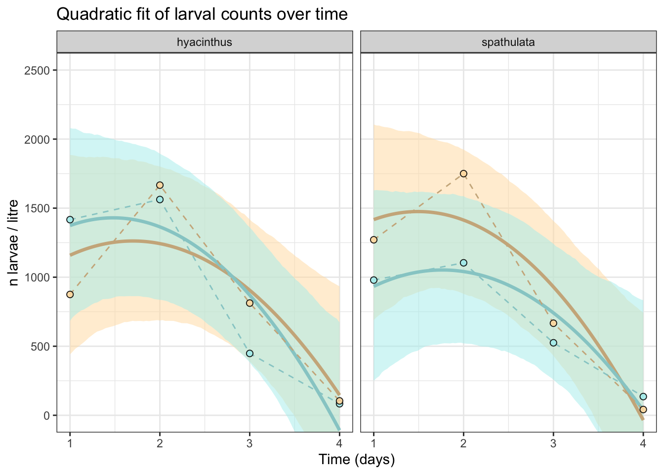
Code
hypothesis(quadratic_counts, "treatmentunimpacted + ItimeE2:treatmentunimpacted = 0")Hypothesis Tests for class b:
Hypothesis Estimate Est.Error CI.Lower CI.Upper Evid.Ratio
1 (treatmentunimpac... = 0 215.11 457.61 -717.78 1165.8 NA
Post.Prob Star
1 NA
---
'CI': 90%-CI for one-sided and 95%-CI for two-sided hypotheses.
'*': For one-sided hypotheses, the posterior probability exceeds 95%;
for two-sided hypotheses, the value tested against lies outside the 95%-CI.
Posterior probabilities of point hypotheses assume equal prior probabilities.No strong evidence of a treatment effect in spathulata.
Estimate 456.2 [–483.5, +1409.8]
Code
hypothesis(quadratic_counts,
  "treatmentunimpacted +
   ItimeE2:treatmentunimpacted +
   treatmentunimpacted:speciesspathulata +
   ItimeE2:treatmentunimpacted:speciesspathulata = 0")
Hypothesis Tests for class b:
Hypothesis Estimate Est.Error CI.Lower CI.Upper Evid.Ratio
1 (treatmentunimpac... = 0 -483.54 456.21 -1409.84 430.19 NA
Post.Prob Star
1 NA
---
'CI': 90%-CI for one-sided and 95%-CI for two-sided hypotheses.
'*': For one-sided hypotheses, the posterior probability exceeds 95%;
for two-sided hypotheses, the value tested against lies outside the 95%-CI.
Posterior probabilities of point hypotheses assume equal prior probabilities.No strong evidence of a treatment effect in hyacinthus.
Estimate –456.21 [–1409.84, 430.191]
Larval settlement (5 days)
Code
#| class-source: fold-hide
#| message: false
#| warning: false
#| fig-width: 9.5
#| fig-height: 5


tiles <- readxl::read_excel("/Users/rof011/reefspawn/code/SurvExpData.xlsx", sheet = "SetTilesSurvREEF_cleaned") |>
  janitor::clean_names() |>
  mutate(days = date_scored - date_tile_deployment) |>
  group_by(plot_id, days, tile_face, treatment, tile_number) |>
  summarise(total_count = sum(settler_count)) |>
  mutate(days = as.numeric(days)) |>
  mutate(days = ifelse(days <100, "5 days", "110 days")) |>
  mutate(days = as.factor(days)) |>
  filter(treatment %in% c("Normal", "Survivor")) |>
  dplyr::mutate(
    treatment = dplyr::case_when(
      stringr::str_detect(treatment, "Survivor") ~ "impacted",
      stringr::str_detect(treatment, "Normal") ~ "unimpacted",
      TRUE ~ NA_character_
    )
  )


tiles_grouped <- tiles |>
  group_by(days, treatment, plot_id, tile_number) |>
  summarise(total_count = sum(total_count))

tiles_grouped_mean <- tiles_grouped |>
  group_by(days, treatment) |>
  summarise(total_count = mean(total_count))

### first timepoint

tiles_counts_a <- brm(
  total_count ~ treatment + (1|plot_id),
  data = tiles_grouped |> filter(days == "5 days"),
  family = gaussian(),
  chains = 4, cores = 4
)

# saveRDS(tiles_counts_a, "/Users/rof011/reefspawn/code/tiles_counts_a.rds")

tiles_counts_a <- readRDS("/Users/rof011/reefspawn/code/tiles_counts_a.rds")

# Create prediction grid
tiles_counts_a_newdata <- expand.grid(
  treatment = unique(tiles_grouped$treatment),
  plot_id = NA  # marginalize over random effect
)

# Get fitted values on response scale with uncertainty
tiles_counts_a_fitted_vals <- fitted(tiles_counts_a, newdata = tiles_counts_a_newdata, scale = "response", allow_new_levels = TRUE) |> as_tibble()
tiles_counts_a_newdata <- bind_cols(tiles_counts_a_newdata, tiles_counts_a_fitted_vals)

#
# ggplot() +
#   theme_bw() +
#   geom_point(data = tiles_grouped |> filter(days == "5 days"), aes(x = treatment, y = total_count, fill = treatment),
#              shape = 21, color = "black", alpha = 0.5, size = 2, position = position_jitter(width = 0.1)) +
#   geom_pointrange(data = tiles_counts_a_newdata,
#                   aes(x = treatment, y = Estimate, ymin = Q2.5, ymax = Q97.5, fill = treatment),
#                   shape = 21, color = "black", size = 1.2) +
#   labs(title = "Predicted settler counts by treatment (ZIP model)",
#        y = "Predicted count (mean ± 95% CI)", x = "Treatment") +
#   scale_fill_manual(values = c("paleturquoise", "navajowhite"))

tileplot_a <- ggplot() + theme_bw() + facet_wrap(~days) +
  geom_violin(data = tiles_grouped |> filter(days == "5 days"), aes(treatment, total_count, fill=treatment), linewidth=0.25, alpha=0.2, show.legend = FALSE) +
  geom_jitter(data = tiles_grouped |> filter(days == "5 days"), aes(treatment, total_count), width=0.1, size=0.4, alpha=0.2, show.legend = FALSE) +
  geom_pointrange(data = tiles_counts_a_newdata,
                  aes(x = treatment, y = Estimate, ymin = Q2.5, ymax = Q97.5, fill = treatment),
                  shape = 21, linewidth=0.5, color = "black", size = 0.6, show.legend = FALSE) +
  scale_fill_manual(values = c("paleturquoise", "navajowhite")) + ylab("Larvae per tile")

tileplot_a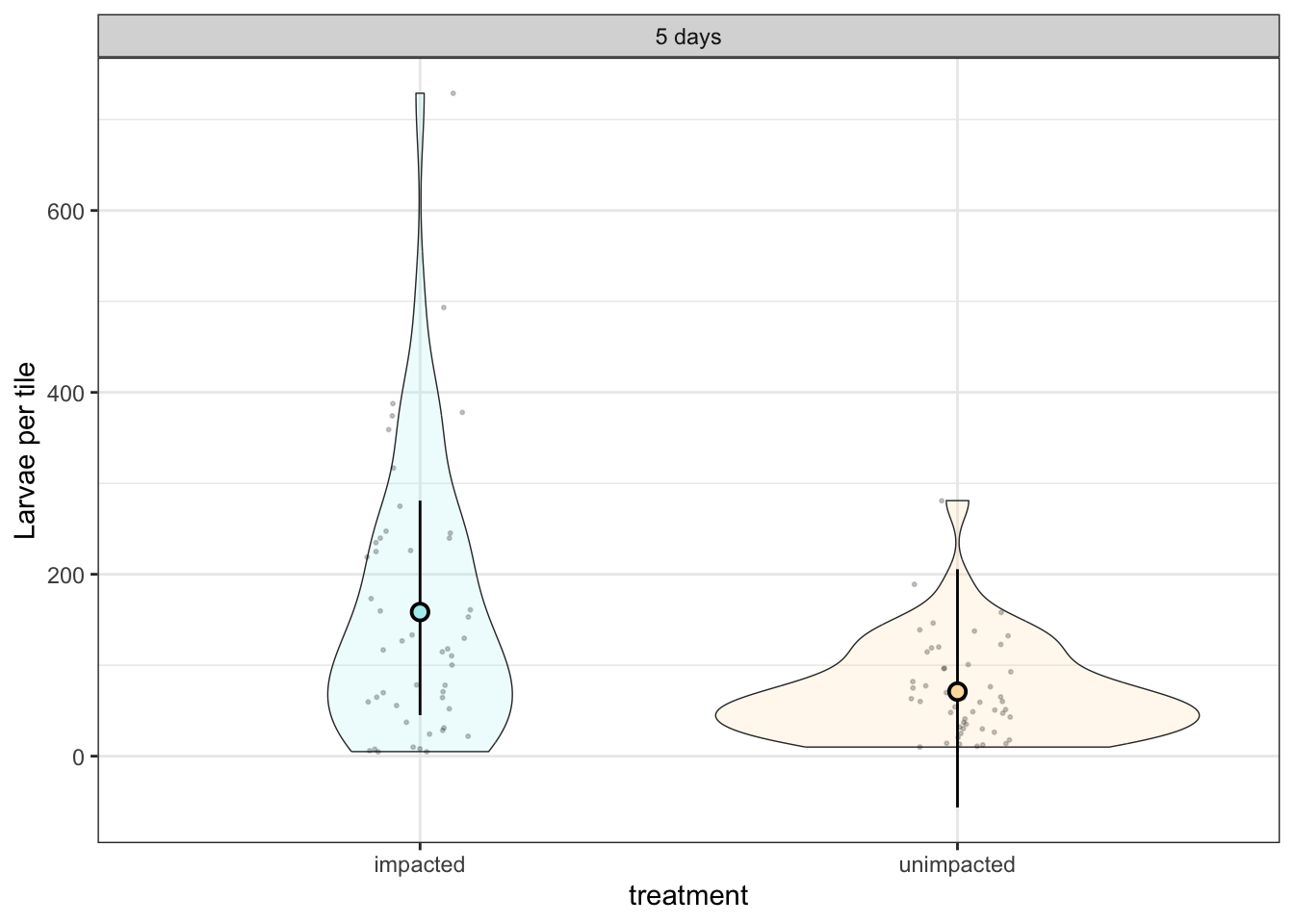
Code
hypothesis(tiles_counts_a, "treatmentunimpacted = 0")Hypothesis Tests for class b:
Hypothesis Estimate Est.Error CI.Lower CI.Upper Evid.Ratio
1 (treatmentunimpac... = 0 -87.49 47.36 -176.56 4.67 NA
Post.Prob Star
1 NA
---
'CI': 90%-CI for one-sided and 95%-CI for two-sided hypotheses.
'*': For one-sided hypotheses, the posterior probability exceeds 95%;
for two-sided hypotheses, the value tested against lies outside the 95%-CI.
Posterior probabilities of point hypotheses assume equal prior probabilities.There is some evidence that unimpacted reefs had lower settler counts than impacted reefs. The effect size is large (–87), but uncertain — CI includes small positive values
Estimate -87.5 [–176.6, +4.7]
Larval recruitment (3 months)
Code
#| class-source: fold-hide
#| message: false
#| warning: false
#| fig-width: 9.5
#| fig-height: 5


# tiles_counts_b <- brm(
#   total_count ~ treatment + (1|plot_id),
#   data = tiles_grouped |> filter(days == "110 days"),
#   family = zero_inflated_poisson(),
#   chains = 4, cores = 4, adapt_delta = 0.95:
# )
#
# saveRDS(tiles_counts_b, "/Users/rof011/reefspawn/code/tiles_counts_b.rds")

tiles_counts_b <- readRDS("/Users/rof011/reefspawn/code/tiles_counts_b.rds")


# Create prediction grid
tiles_counts_b_newdata <- expand.grid(
  treatment = unique(tiles_grouped$treatment),
  plot_id = NA  # marginalize over random effect
)

# Get fitted values on response scale with uncertainty
tiles_counts_b_fitted_vals <- fitted(tiles_counts_b, newdata = tiles_counts_b_newdata, scale = "response", allow_new_levels = TRUE) |> as_tibble()
tiles_counts_b_newdata <- bind_cols(tiles_counts_b_newdata, tiles_counts_b_fitted_vals)

#
# tileplot_b <- ggplot() +
#   theme_bw() +
#   geom_point(data = tiles_grouped |> filter(days == "5 days"), aes(x = treatment, y = total_count, fill = treatment),
#              shape = 21, color = "black", alpha = 0.5, size = 2, position = position_jitter(width = 0.1)) +
#   geom_pointrange(data = tiles_counts_b_newdata,
#                   aes(x = treatment, y = Estimate, ymin = Q2.5, ymax = Q97.5, fill = treatment),
#                   shape = 21, color = "black", size = 1.2) +
#   labs(title = "Predicted settler counts by treatment (ZIP model)",
#        y = "Predicted count (mean ± 95% CI)", x = "Treatment") +
#   scale_fill_manual(values = c("paleturquoise", "navajowhite"))

tileplot_b <- ggplot() + theme_bw() + facet_wrap(~days) +
  geom_violin(data = tiles_grouped |> filter(days == "110 days"), aes(treatment, total_count, fill=treatment), linewidth=0.25, alpha=0.2, show.legend = FALSE) +
  geom_jitter(data = tiles_grouped |> filter(days == "110 days"), aes(treatment, total_count), width=0.1, size=0.4, alpha=0.2, show.legend = FALSE) +
  geom_pointrange(data = tiles_counts_b_newdata,
                  aes(x = treatment, y = Estimate, ymin = Q2.5, ymax = Q97.5, fill = treatment),
                  shape = 21, linewidth=0.5, stroke = 0.5, color = "black", size = 0.6, show.legend = FALSE) +
  scale_fill_manual(values = c("paleturquoise", "navajowhite")) + ylab("Larvae per tile")

tileplot_b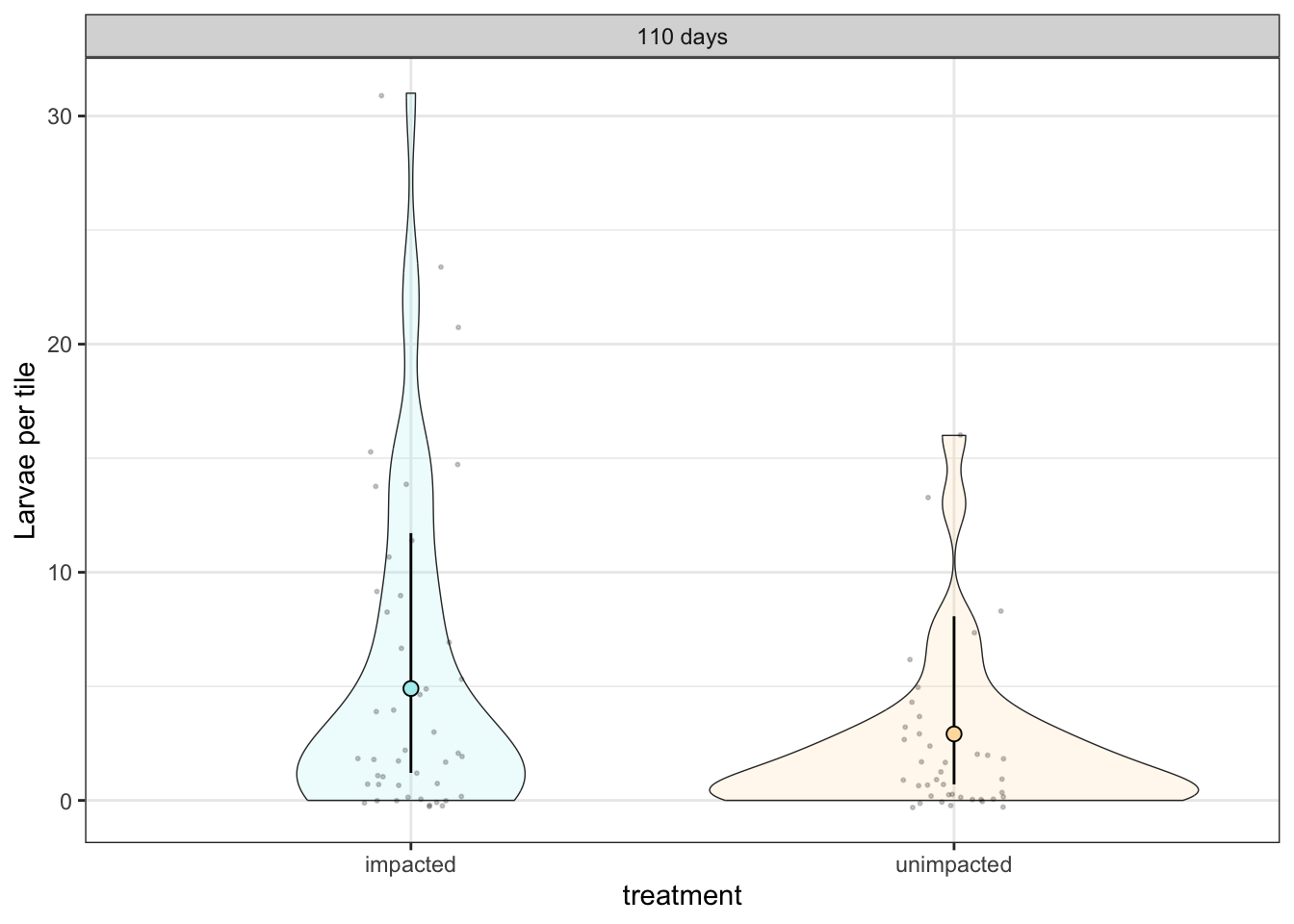
Code
hypothesis(tiles_counts_b, "treatmentunimpacted = 0")Hypothesis Tests for class b:
Hypothesis Estimate Est.Error CI.Lower CI.Upper Evid.Ratio
1 (treatmentunimpac... = 0 -0.52 0.47 -1.42 0.43 NA
Post.Prob Star
1 NA
---
'CI': 90%-CI for one-sided and 95%-CI for two-sided hypotheses.
'*': For one-sided hypotheses, the posterior probability exceeds 95%;
for two-sided hypotheses, the value tested against lies outside the 95%-CI.
Posterior probabilities of point hypotheses assume equal prior probabilities.No strong evidence of a treatment effect
Estimate 0.52 [–1.42, +0.43]
Posterior predictions
i) effect sizes (impacted vs unimpacted)
proportional effect sizes, calculated as:
where:
•   1 = no effect (impacted = unimpacted)
•   <1 = negative effect (impacted < unimpacted)
•   >1 = positive effect (impacted > unimpacted)
Code
##############################
##### fm_egg_size
##############################

posterior <- as.data.frame(fm_egg_size)
mu_hyacinthus_impacted <- posterior$b_Intercept
mu_hyacinthus_unimpacted <- posterior$b_Intercept + posterior$b_treatmentunimpacted
mu_spathulata_impacted <- posterior$b_Intercept + posterior$`b_speciesspathulatha`
mu_spathulata_unimpacted <- mu_spathulata_impacted +
  posterior$`b_treatmentunimpacted` +
  posterior$`b_treatmentunimpacted:speciesspathulatha`

rel_pct_hyacinthus <- (mu_hyacinthus_impacted / mu_hyacinthus_unimpacted)
rel_pct_spathulata <- (mu_spathulata_impacted / mu_spathulata_unimpacted)

fm_egg_size_posterior <- tibble(
  species = c("hyacinthus", "spathulata"),
  effect_size = c(mean(rel_pct_hyacinthus), mean(rel_pct_spathulata)) - 1,
  effect_lower = c(quantile(rel_pct_hyacinthus, 0.025), quantile(rel_pct_spathulata, 0.025)) - 1,
  effect_upper = c(quantile(rel_pct_hyacinthus, 0.975), quantile(rel_pct_spathulata, 0.975)) - 1
) |> mutate(stage = "1. oocyte size")


##############################
##### fm_reproductive_output
##############################

posterior_repro <- as.data.frame(fm_reproductive_output)
mu_hyacinthus_impacted <- posterior_repro$b_Intercept
mu_hyacinthus_unimpacted <- posterior_repro$b_Intercept + posterior_repro$b_treatmentunimpacted
mu_spathulata_impacted <- posterior_repro$b_Intercept + posterior_repro$`b_speciesspathulatha`
mu_spathulata_unimpacted <- mu_spathulata_impacted +
  posterior_repro$`b_treatmentunimpacted` +
  posterior_repro$`b_treatmentunimpacted:speciesspathulatha`

rel_pct_hyacinthus <- (mu_hyacinthus_impacted / mu_hyacinthus_unimpacted)
rel_pct_spathulata <- (mu_spathulata_impacted / mu_spathulata_unimpacted)

fm_repro_posterior <- tibble(
  species = c("hyacinthus", "spathulata"),
  effect_size = c(mean(rel_pct_hyacinthus), mean(rel_pct_spathulata)) - 1,
  effect_lower = c(quantile(rel_pct_hyacinthus, 0.025), quantile(rel_pct_spathulata, 0.025)) - 1,
  effect_upper = c(quantile(rel_pct_hyacinthus, 0.975), quantile(rel_pct_spathulata, 0.975)) - 1
) |> mutate(stage = "2. reproductive biomass")


##############################
##### larval development
##############################

posterior <- as.data.frame(quadratic_counts)
time <- 1.5
time2 <- time^2

mu_h_impacted <- posterior$b_Intercept + posterior$b_time * time + posterior$`b_ItimeE2` * time2
mu_h_unimpacted <- mu_h_impacted + posterior$`b_treatmentunimpacted` + posterior$`b_ItimeE2:treatmentunimpacted` * time2
mu_s_impacted <- mu_h_impacted + posterior$`b_speciesspathulata` + posterior$`b_ItimeE2:speciesspathulata` * time2
mu_s_unimpacted <- mu_s_impacted +
  posterior$`b_treatmentunimpacted` +
  posterior$`b_ItimeE2:treatmentunimpacted` * time2 +
  posterior$`b_treatmentunimpacted:speciesspathulata` +
  posterior$`b_ItimeE2:treatmentunimpacted:speciesspathulata` * time2

rel_pct_h <- mu_h_impacted /mu_h_unimpacted
rel_pct_s <- mu_s_impacted / mu_s_unimpacted

quadratic_counts_posterior <- tibble(
  species = c("hyacinthus", "spathulata"),
  effect_size = c(mean(rel_pct_h), mean(rel_pct_s)) - 1,
  effect_lower = c(quantile(rel_pct_h, 0.025), quantile(rel_pct_s, 0.025)) - 1,
  effect_upper = c(quantile(rel_pct_h, 0.975), quantile(rel_pct_s, 0.975)) - 1
) |> mutate(stage = "3. larval development")


##############################
##### larval settlement
##############################

posterior <- as.data.frame(tiles_counts_a)
mu_impacted <- posterior$b_Intercept
mu_unimpacted <- mu_impacted + posterior$b_treatmentunimpacted
rel_pct <- mu_impacted/ mu_unimpacted

tiles_counts_a_posterior <- tibble(
  effect_size = mean(rel_pct) - 1,
  effect_lower = quantile(rel_pct, 0.025) - 1,
  effect_upper = quantile(rel_pct, 0.975) - 1,
  species = NA,
  stage = "4. larval settlement"
)


##############################
##### larval recruitment
##############################

posterior <- as.data.frame(tiles_counts_b)
log_mu_impacted <- posterior$b_Intercept
log_mu_unimpacted <- log_mu_impacted + posterior$b_treatmentunimpacted
mu_impacted <- exp(log_mu_impacted)
mu_unimpacted <- exp(log_mu_unimpacted)
rel_pct <-  mu_impacted / mu_unimpacted

tiles_counts_b_posterior <- tibble(
  effect_size = mean(rel_pct) - 1,
  effect_lower = quantile(rel_pct, 0.025) - 1,
  effect_upper = quantile(rel_pct, 0.975) - 1,
  species = NA,
  stage = "5. larval recruitment"
)


##############################
##### Combine
##############################

posterior_prediction_table <- bind_rows(
  fm_egg_size_posterior,
  fm_repro_posterior,
  quadratic_counts_posterior,
  tiles_counts_a_posterior,
  tiles_counts_b_posterior
) |>
  mutate(across(c(effect_size, effect_lower, effect_upper), ~ round(.x, 1))) |>
  mutate(across(c(effect_size, effect_lower, effect_upper), ~ as.numeric(.x))) |>
  mutate(species = ifelse(is.na(species), "pooled", species)) |>
  select(stage, species, effect_size, effect_lower, effect_upper) |>
  arrange(stage, species)

blankdf <- data.frame(
    stage =c("4. larval settlement",  "5. larval recruitment"),
    species = NA, effect_size = NA, effect_lower = NA, effect_upper = NA)

DT::datatable(
  posterior_prediction_table,
  rownames = FALSE,
  options = list(
    pageLength = 10,
    autoWidth = TRUE,
    dom = 't'
  ),
  class = 'stripe hover compact',
  escape = FALSE
) %>%
  DT::formatStyle(
    columns = names(posterior_prediction_table),
    fontSize = '70%'
  ) %>%
  DT::formatStyle(
    'stage',
    target = 'row',
    backgroundColor = DT::styleEqual(
      unique(posterior_prediction_table$stage),
      gray.colors(length(unique(posterior_prediction_table$stage)), start = 0.9, end = 0.7)
    )
  )
Code
posterior_prediction_table_full <- rbind(posterior_prediction_table, blankdf)

posterior_predicts <- ggplot() +
  theme_bw() +
  facet_grid(~stage, scales = "free") +
  geom_col(data = posterior_prediction_table_full,
           aes(x = stage, y = effect_size, group = species, fill = species),
           position = position_dodge(width = 0.45), width = 0.4, col="black", linewidth=0.2) +
  geom_errorbar(data = posterior_prediction_table_full,
                aes(x = stage, y = effect_size, group = species, ymin = effect_lower, ymax = effect_upper),
                width = 0.1, position = position_dodge(width = 0.45)) +
  scale_y_continuous(limits = c(-2.5, 2.5), breaks=c(-2, -1, 1, 2), oob = scales::oob_keep) +
  labs(x = NULL, y = "Effect size (log scale difference)", fill = "Species") +
  geom_hline(yintercept = 0, linewidth=0.2) +
  theme(panel.grid.major.x = element_blank(),
        panel.grid.minor.x = element_blank())

posterior_predicts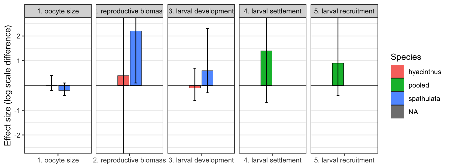
Code
#ggsave(posterior_predicts,filename="/Users/rof011/reefspawn/code/posterior_predicts.pdf", width=6, height=2)ii) cumulative effects across life history stages
The cumulative effect size is the product of all individual stage posteriors:
Code
posterior_prediction_table <- bind_rows(
  fm_egg_size_posterior,
  fm_repro_posterior,
  quadratic_counts_posterior,
  tiles_counts_a_posterior,
  tiles_counts_b_posterior
) |>
  mutate(across(c(effect_size, effect_lower, effect_upper), ~ round(.x, 1))) |>
  mutate(across(c(effect_size, effect_lower, effect_upper), ~ as.numeric(.x))) |>
  mutate(species = ifelse(is.na(species), "pooled", species)) |>
  select(stage, species, effect_size, effect_lower, effect_upper) |>
  arrange(stage, species)

pooled_vals <- posterior_prediction_table |>
  filter(species == "pooled")

blankdf <- pooled_vals |>
  slice(rep(1:n(), each = 2)) |>
  mutate(species = rep(c("hyacinthus", "spathulata"), times = nrow(pooled_vals)))

posterior_prediction_table <- rbind(posterior_prediction_table |> filter(!species=="pooled"), blankdf) |>
  arrange(stage, species)

posterior_prediction_table_wider <- posterior_prediction_table |>
  select(stage, species, effect_size) |>
  pivot_wider(names_from = "stage", values_from = "effect_size") |>
  rename(oocyte=2, biomass=3, larvae=4, settlement=5, recruitment=6) |>
  mutate(probability = oocyte*biomass*larvae*settlement*recruitment)


#### posterior
# ========================
# 1. Extract posteriors
# ========================

posterior_egg     <- as.data.frame(fm_egg_size)
posterior_repro   <- as.data.frame(fm_reproductive_output)
posterior_dev     <- as.data.frame(quadratic_counts)
posterior_settle  <- as.data.frame(tiles_counts_a)
posterior_recruit <- as.data.frame(tiles_counts_b)

# ========================
# 2. Posterior ratios
# ========================

## Egg size
rel_pct_egg_h <- posterior_egg$b_Intercept / (posterior_egg$b_Intercept + posterior_egg$b_treatmentunimpacted)
rel_pct_egg_s <- (posterior_egg$b_Intercept + posterior_egg$`b_speciesspathulatha`) /
  (posterior_egg$b_Intercept + posterior_egg$`b_speciesspathulatha` +
   posterior_egg$b_treatmentunimpacted + posterior_egg$`b_treatmentunimpacted:speciesspathulatha`)

## Reproductive output
rel_pct_repro_h <- posterior_repro$b_Intercept / (posterior_repro$b_Intercept + posterior_repro$b_treatmentunimpacted)
rel_pct_repro_s <- (posterior_repro$b_Intercept + posterior_repro$`b_speciesspathulatha`) /
  (posterior_repro$b_Intercept + posterior_repro$`b_speciesspathulatha` +
   posterior_repro$b_treatmentunimpacted + posterior_repro$`b_treatmentunimpacted:speciesspathulatha`)

## Larval development
time <- 1.5
time2 <- time^2
mu_h_impacted <- posterior_dev$b_Intercept + posterior_dev$b_time * time + posterior_dev$`b_ItimeE2` * time2
mu_h_unimpacted <- mu_h_impacted + posterior_dev$b_treatmentunimpacted + posterior_dev$`b_ItimeE2:treatmentunimpacted` * time2

mu_s_impacted <- mu_h_impacted + posterior_dev$`b_speciesspathulata` + posterior_dev$`b_ItimeE2:speciesspathulata` * time2
mu_s_unimpacted <- mu_s_impacted +
  posterior_dev$b_treatmentunimpacted +
  posterior_dev$`b_ItimeE2:treatmentunimpacted` * time2 +
  posterior_dev$`b_treatmentunimpacted:speciesspathulata` +
  posterior_dev$`b_ItimeE2:treatmentunimpacted:speciesspathulata` * time2

rel_pct_dev_h <- mu_h_impacted / mu_h_unimpacted
rel_pct_dev_s <- mu_s_impacted / mu_s_unimpacted

## Settlement (pooled)
rel_pct_settle <- posterior_settle$b_Intercept / (posterior_settle$b_Intercept + posterior_settle$b_treatmentunimpacted)

## Recruitment (pooled, log-link)
mu_impacted <- exp(posterior_recruit$b_Intercept)
mu_unimpacted <- exp(posterior_recruit$b_Intercept + posterior_recruit$b_treatmentunimpacted)
rel_pct_recruit <- mu_impacted / mu_unimpacted

# ========================
# 3. Combine and summarise
# ========================

combined_draws_h <- mean(rel_pct_egg_h) * mean(rel_pct_repro_h) * mean(rel_pct_dev_h) * mean(rel_pct_settle) * mean(rel_pct_recruit) /5

combined_draws_s <- mean(rel_pct_egg_s) * mean(rel_pct_repro_s) * mean(rel_pct_dev_s) * mean(rel_pct_settle) * mean(rel_pct_recruit) /5


posterior_cumulative <- tibble(
  species = c("hyacinthus", "spathulata"),
  oocyte_size = c(mean(rel_pct_egg_h), mean(rel_pct_egg_s)),
  reproductive_biomass = c(mean(rel_pct_repro_h), mean(rel_pct_repro_s)),
  larval_development = c(mean(rel_pct_dev_h), mean(rel_pct_dev_s)),
  larval_settlement = c(mean(rel_pct_settle), mean(rel_pct_settle)),
  larval_recruitment = c(mean(rel_pct_recruit), mean(rel_pct_recruit)),
  cumulative_effect_size = c(mean(combined_draws_h - 1), mean(combined_draws_s - 1)),
  cumulative_effect_lower = c(quantile(combined_draws_h - 1, 0.025), quantile(combined_draws_s - 1, 0.025)),
  cumulative_effect_upper = c(quantile(combined_draws_h - 1, 0.975), quantile(combined_draws_s - 1, 0.975))
) |>
  mutate(across(where(is.numeric), round, 1)) |>
  select(-cumulative_effect_lower, -cumulative_effect_upper)

posterior_cumulative |>
  DT::datatable(
    options = list(
      pageLength = 5,
      autoWidth = TRUE,
      dom = 't',
      columnDefs = list(
        list(className = 'dt-center', targets = "_all")
      )
    ),
    rownames = FALSE
  ) %>%
  DT::formatStyle(
    columns = names(posterior_cumulative),
    fontSize = '70%'
  ) %>%
  DT::formatStyle(
    'species',
    target = 'row',
    backgroundColor = DT::styleEqual(
      unique(posterior_cumulative$species),
      gray.colors(length(unique(posterior_cumulative$species)), start = 0.9, end = 0.8)
    )
  )
Code
#| class-source: fold-hide
#| message: false
#| warning: false
#| fig-width: 10
#| fig-height: 2
#|


p <- (a + ggtitle("") | b + ggtitle("") | plot_c + ggtitle("") | tileplot_a + ggtitle("") | tileplot_b + ggtitle(""))

ggsave("/Users/rof011/reefspawn/code/patchwork_plot.png", plot = p, width = 50, height = 5, units = "in", dpi = 300, limitsize = FALSE)

#knitr::include_graphics("/Users/rof011/reefspawn/code/patchwork_plot.png")

library(patchwork)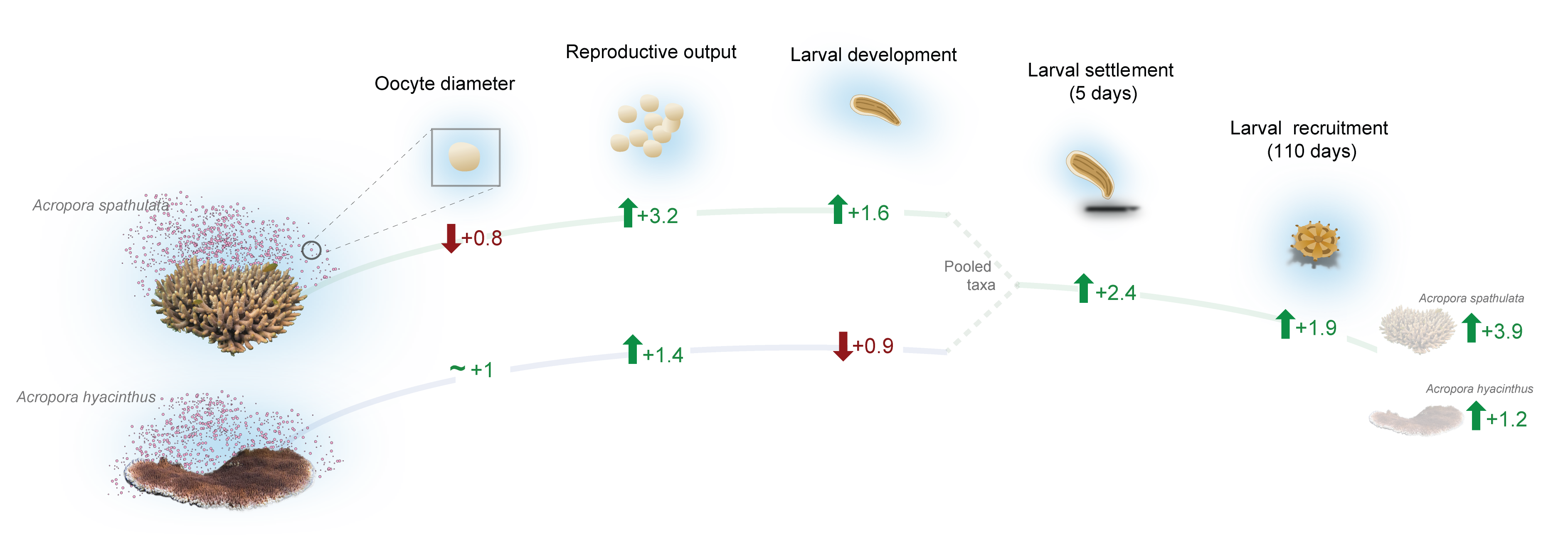
•   1 = no effect (impacted = unimpacted)
•   <1 = negative effect (impacted < unimpacted)
•   >1 = positive effect (impacted > unimpacted)