Bayesian models
1. Parameter estimates
All data sourced from Lizard Island corals via Álvarez-Noriega et al 2016 and Madin et al 2023.
Main data available with package as coralsize:
Code
library(tidyverse)
library(forcats)
library(units)
library(ggplot2)
library(fGarch)
library(brms)


sp_order <- c("Acropora hyacinthus", "Acropora cytherea",
              "Acropora intermedia", "Acropora robusta",
              "Acropora millepora", "Acropora nasuta", "Acropora spathulata",
              "Acropora humilis", "Acropora cf. digitifera",
              "Goniastrea pectinata", "Goniastrea retiformis")


sp_pal <- c("Acropora hyacinthus" = "#50676c", "Acropora cytherea" = "#3a6c8e",
  "Acropora intermedia" = "#2c3687", "Acropora robusta" = "#7b8ca8",
  "Acropora spathulata" = "#98a062", "Acropora millepora" = "#665a43", "Acropora nasuta" =  "#48642f",
  "Acropora humilis" = "#824b3b", "Acropora cf. digitifera" = "#a47c73",
  "Goniastrea pectinata" = "#999999", "Goniastrea retiformis"= "#bfbfbf")

make_paler <- function(color) {
  grDevices::adjustcolor(color, alpha.f = 1, red.f = 1.2, green.f = 1.2, blue.f = 1.2)
}

# Apply the function to the palette
sp_pal <- sapply(sp_pal, make_paler)


size_data <- coralsize |>
  mutate(width=sqrt(area_cm2/pi)*2) |>
  mutate(species=as.factor(species)) |>
  mutate(species=fct_relevel(species,sp_order)) |>
  mutate(growthform=fct_recode(species, "Tabular"= "Acropora cytherea", "Tabular"= "Acropora hyacinthus",
                                        "Branching"= "Acropora intermedia", "Branching"= "Acropora robusta",
                                        "Massive" = "Goniastrea pectinata", "Massive" = "Goniastrea retiformis",
                                        "Corymbose" = "Acropora nasuta", "Corymbose" = "Acropora millepora", "Corymbose" = "Acropora spathulata",
                                        "Digitate" = "Acropora cf. digitifera", "Digitate" = "Acropora humilis"))


ggplot() + theme_bw() + facet_wrap(~growthform, scales="free") +
  geom_density(data=size_data, aes(width, fill=species, color=species), alpha=0.3, linewidth=0.6, show.legend=TRUE) +
  theme(panel.grid = element_blank()) + ylab("") +
  scale_color_manual(values=sp_pal) + scale_fill_manual(values=sp_pal)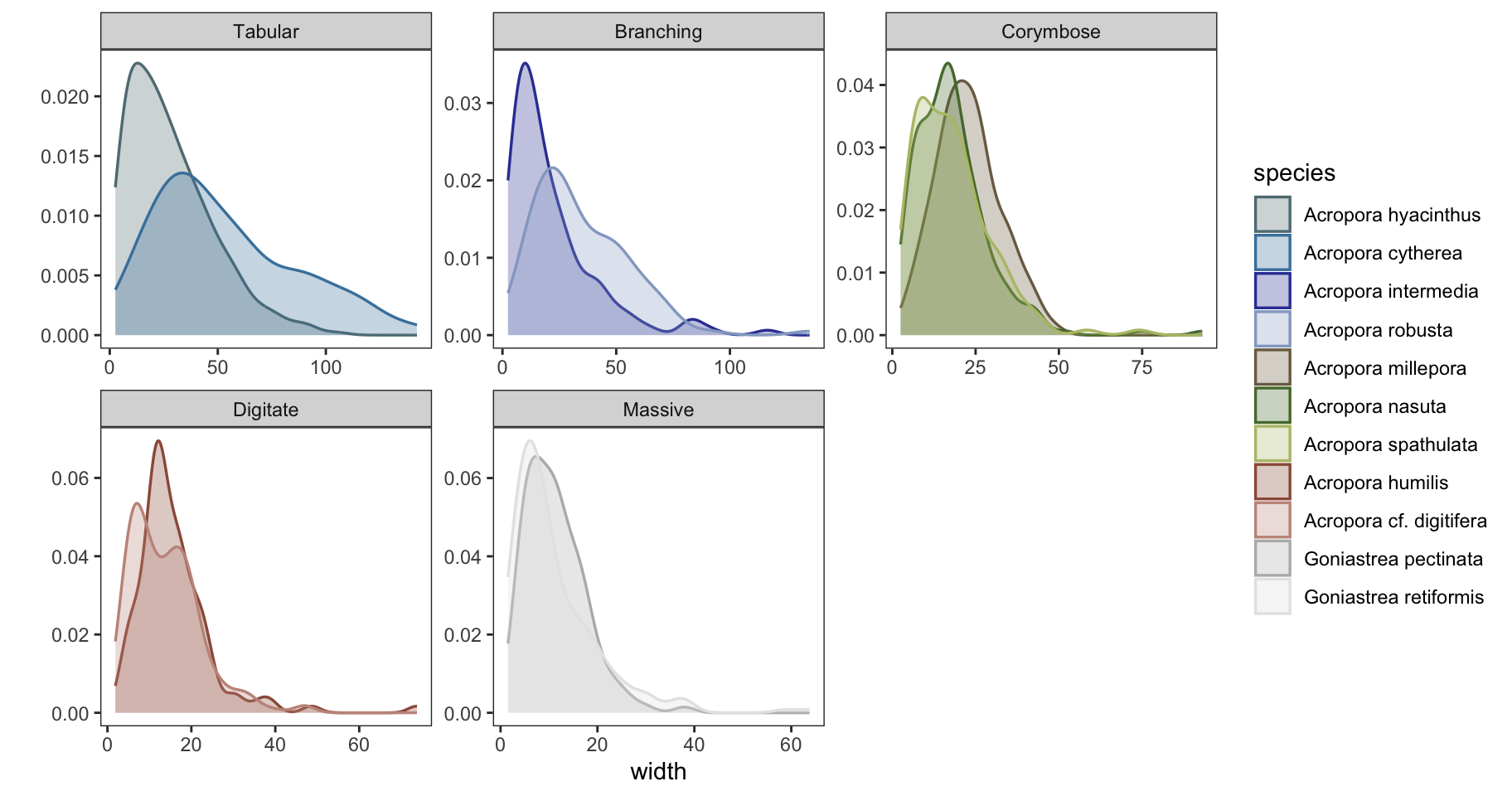
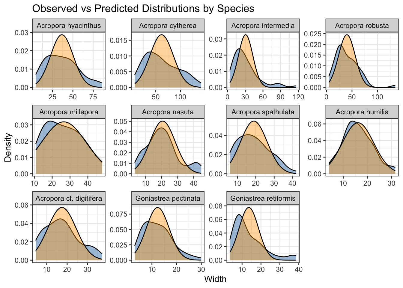
i. Colony size distributions
Data subset to 2011 (last datapoint) to predict size distributions:
plot the fitted distributions (yellow) against the raw data:
fitted_vals <- fitted(brm_sizedistribution, scale = "response")

size_data <- size_data |> filter(year==2011) |> mutate(fitted = fitted(brm_sizedistribution, scale = "response")[, "Estimate"])

ggplot() + theme_bw() + facet_wrap(~species, scales = "free") +
  geom_density(data = size_data, aes(x = width), fill = "steelblue", alpha = 0.5, show.legend=TRUE) +
  geom_density(data = size_data, aes(x = fitted), fill = "orange", alpha = 0.4, show.legend=TRUE) +
  labs(
    x = "Width",
    y = "Density",
    title = "Observed vs Predicted Distributions by Species"
  )
ii. Polyp-level fecundity
Predict the total number of oocytes per species * size:
Extract conditional effects:
Code
brm_fecundity_cond <- conditional_effects(brm_fecundity, effects = "width:species", dpar = "mu")
brm_fecundity_plots <- brm_fecundity_cond$`width:species` |> as.data.frame() %>%
  mutate(species=fct_relevel(species,sp_order)) |>
  mutate(growthform=fct_recode(species, "Tabular"= "Acropora cytherea", "Tabular"= "Acropora hyacinthus",
                                        "Branching"= "Acropora intermedia", "Branching"= "Acropora robusta",
                                        "Massive" = "Goniastrea pectinata", "Massive" = "Goniastrea retiformis",
                                        "Corymbose" = "Acropora nasuta", "Corymbose" = "Acropora millepora",
                                        "Corymbose" = "Acropora spathulata",
                                        "Digitate" = "Acropora cf. digitifera", "Digitate" = "Acropora humilis"))

ggplot() + theme_bw() + facet_wrap(~growthform, scales="free_y") + ylab("oocytes per polyp") +
  geom_line(data=brm_fecundity_plots, aes(width, estimate__, color=species), show.legend=TRUE) +
  geom_ribbon(data=brm_fecundity_plots, aes(width, ymin=lower__, ymax=upper__, fill=species), alpha=0.2, show.legend=TRUE) +
  scale_color_manual(values=sp_pal) + scale_fill_manual(values=sp_pal)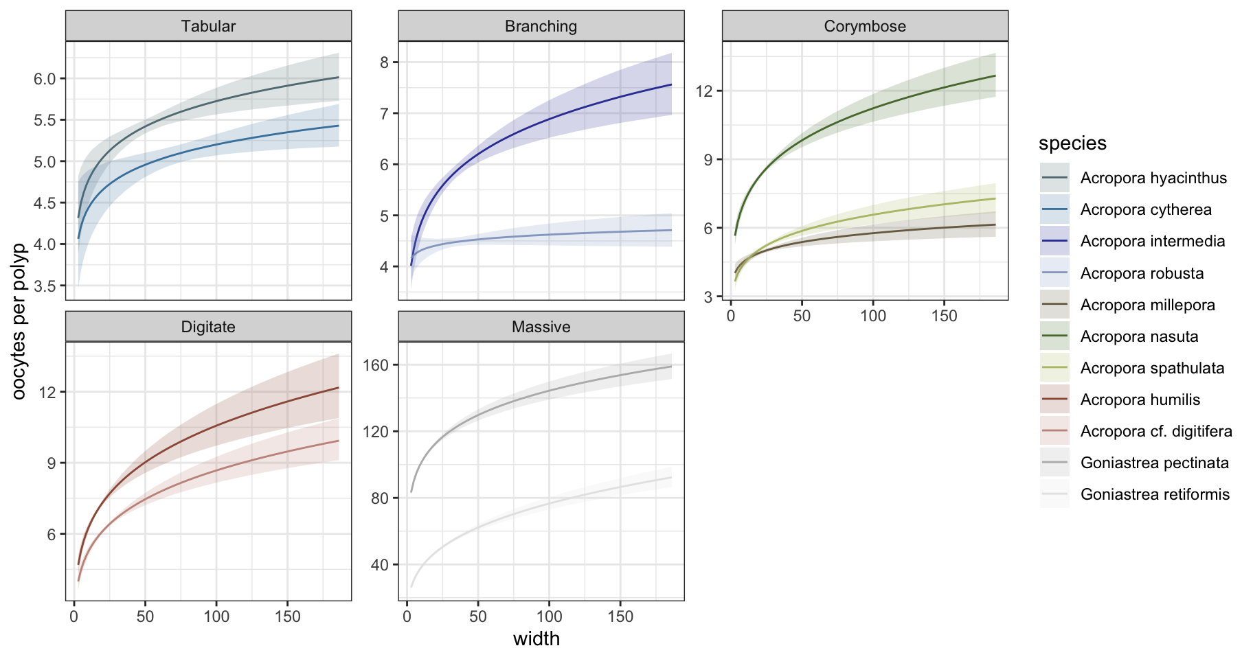
iii. Colony-level fecundity
Predict the probability of fecundity per species (binary depending on colony size:
Extract conditional effects:
Code
#| class-source: fold-hide
#| message: false
#| warning: false
#| fig-width: 9.5
#| fig-height: 5

brm_probability_cond <- conditional_effects(brm_probability, effects = "width:species", dpar = "mu")
brm_probability_plots <-  brm_probability_cond$`width:species` |> as.data.frame() %>%
  mutate(growthform=fct_recode(species, "Tabular"= "Acropora cytherea", "Tabular"= "Acropora hyacinthus",
                                        "Branching"= "Acropora intermedia", "Branching"= "Acropora robusta",
                                        "Massive" = "Goniastrea pectinata", "Massive" = "Goniastrea retiformis",
                                        "Corymbose" = "Acropora nasuta", "Corymbose" = "Acropora millepora", "Corymbose" = "Acropora spathulata",
                                        "Digitate" = "Acropora cf. digitifera", "Digitate" = "Acropora humilis"))

ggplot() + theme_bw() + facet_wrap(~growthform, scales="free_y") +
  geom_line(data=brm_probability_plots, aes(width, estimate__, color=species), show.legend=TRUE) +
  geom_ribbon(data=brm_probability_plots, aes(width, ymin=lower__, ymax=upper__, fill=species), alpha=0.2, show.legend=TRUE) +
    scale_color_manual(values=sp_pal) + scale_fill_manual(values=sp_pal) +
  ylab("Probability of reproductive colonies") + xlab("Colony width")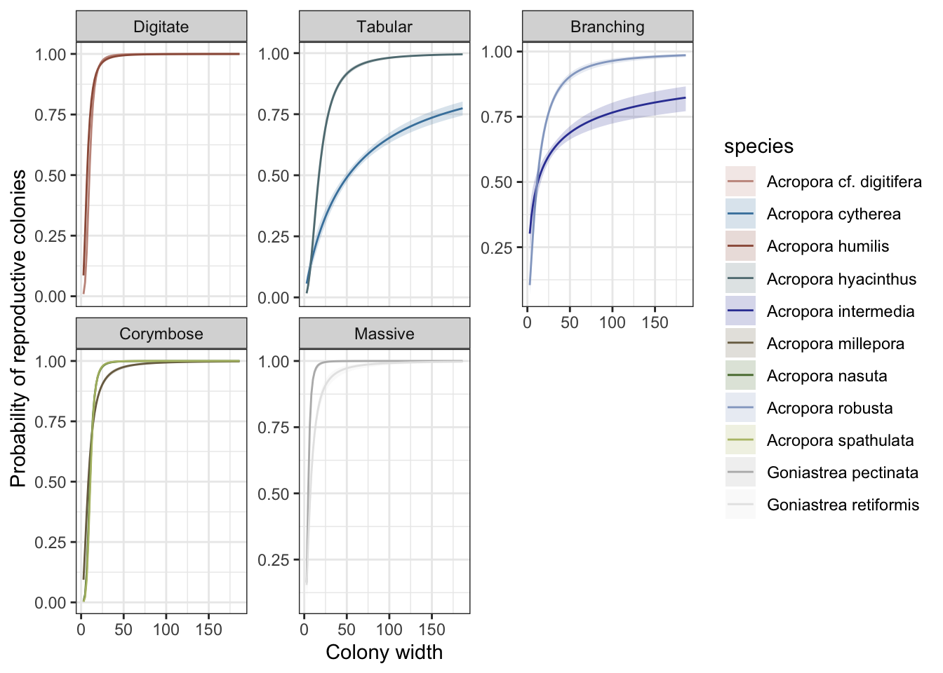
iv. Colony-level polyp density
Predict the probability of density of polyps per cm^2 per species:
brm_polyp_density <- brm(cm2 ~ species,
                         family = gaussian,
                         iter = 10000,
                         chains = 8,
                         cores = 11,
                         data=polyp_density_data)
Extract conditional effects:
Code
# add a hack to get millepora, assume it's between millepora and nasuta
millepora <- polyp_density_data |> filter(species=="Acropora nasuta" | species=="Acropora spathulata") |>
                mutate(species="Acropora millepora") |>
                mutate(spp = "AM")

# rejoin
polyp_density_data <- polyp_density_data |> rbind(millepora) |>
  mutate(growthform=fct_recode(species, "Tabular"= "Acropora cytherea", "Tabular"= "Acropora hyacinthus",
                                        "Branching"= "Acropora intermedia", "Branching"= "Acropora robusta",
                                        "Massive" = "Goniastrea pectinata", "Massive" = "Goniastrea retiformis",
                                        "Corymbose" = "Acropora nasuta", "Corymbose" = "Acropora millepora",
                                        "Corymbose" = "Acropora spathulata",
                                        "Digitate" = "Acropora cf. digitifera", "Digitate" = "Acropora humilis"))

### data prep above for the brms model


brm_polyp_density_cond <- conditional_effects(brm_polyp_density, effects = "species", dpar = "mu")

brm_probability_plots <-  brm_polyp_density_cond$species |> as.data.frame() %>%
  mutate(growthform=fct_recode(species, "Tabular"= "Acropora cytherea", "Tabular"= "Acropora hyacinthus",
                                        "Branching"= "Acropora intermedia", "Branching"= "Acropora robusta",
                                        "Massive" = "Goniastrea pectinata", "Massive" = "Goniastrea retiformis",
                                        "Corymbose" = "Acropora nasuta", "Corymbose" = "Acropora millepora", "Corymbose" = "Acropora spathulata",
                                        "Digitate" = "Acropora cf. digitifera", "Digitate" = "Acropora humilis"))

ggplot() + theme_bw() + facet_wrap(~growthform, scales="free") +
  geom_col(data=brm_probability_plots, aes(species, estimate__, fill=species),
           color="black", alpha=0.5, linewidth=0.5, show.legend=FALSE) +
  geom_errorbar(data=brm_probability_plots, aes(species, estimate__, ymin=lower__, ymax=upper__, fill=species),
                width=0.05, color="black", alpha=0.8, linewidth=0.5, show.legend=FALSE) +
  theme(axis.text.x = element_text(angle = 45, vjust = 0.9, hjust=0.8)) +
  scale_color_manual(values=sp_pal) + scale_fill_manual(values=sp_pal) +
  ylab(bquote('Polyps per'*~cm^2*'')) + xlab("")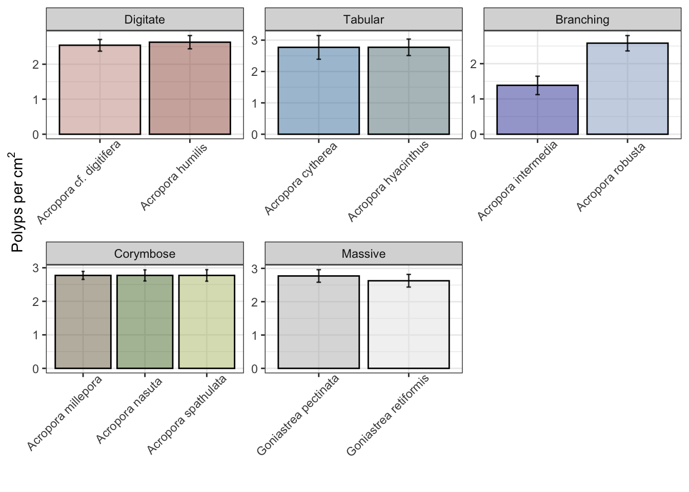
v. Colony-level reproductive area
Predict the proportion of coral area that is reproductive (not within sterile growth zone at borders):
Code
sterile_zone <- tibble(
       species = c("Acropora hyacinthus", "Acropora cytherea", "Acropora cf. digitifera",
                  "Acropora humilis", "Acropora nasuta", "Acropora spathulata",
                  "Acropora millepora","Acropora intermedia","Acropora robusta"),
       lower__ = c(0.760, 0.999, 0.773, 0.995, 0.970, 0.885, 0.885, 0.760, 0.760),
       median = c(0.771, 1.000, 0.868, 1.000, 0.999, 0.913, 0.913, 0.771, 0.771),
       upper__ = c(0.781, 1.000, 0.936, 1.000, 1.000, 0.941, 0.941, 0.781, 0.781)
        )  |>
  mutate(growthform=fct_recode(species, "Tabular"= "Acropora cytherea", "Tabular"= "Acropora hyacinthus",
                                        "Branching"= "Acropora intermedia", "Branching"= "Acropora robusta",
                                        "Corymbose" = "Acropora nasuta", "Corymbose" = "Acropora millepora", "Corymbose" = "Acropora spathulata",
                                        "Digitate" = "Acropora cf. digitifera", "Digitate" = "Acropora humilis")) |>
  bind_rows(data.frame(species = c("Goniastrea retiformis", "Goniastrea pectinata"),
                                          lower__ = c(1,1),
                                          median = c(1,1),
                                          upper__ = c(1,1),
                                          growthform = c("Massive","Massive")))

ggplot() + theme_bw() + facet_wrap(~growthform, scales="free_x") +
  geom_col(data=sterile_zone, aes(species, median*100, fill=species),
           color="black", alpha=0.3, linewidth=0.5, show.legend=FALSE) +
  geom_errorbar(data=sterile_zone, aes(species, median*100, ymin=lower__*100, ymax=upper__*100),
                width=0.05, color="black", alpha=0.8, linewidth=0.5, show.legend=FALSE) +
  theme(axis.text.x = element_text(angle = 45, vjust = 0.9, hjust=0.8)) +
  scale_color_manual(values=sp_pal) + scale_fill_manual(values=sp_pal) +
  ylab("Proportion colony reproductive") + xlab("")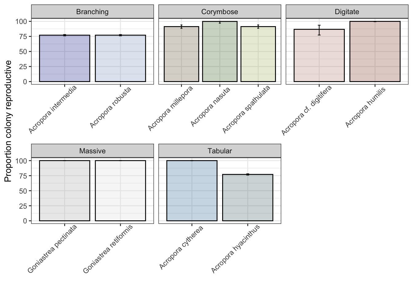
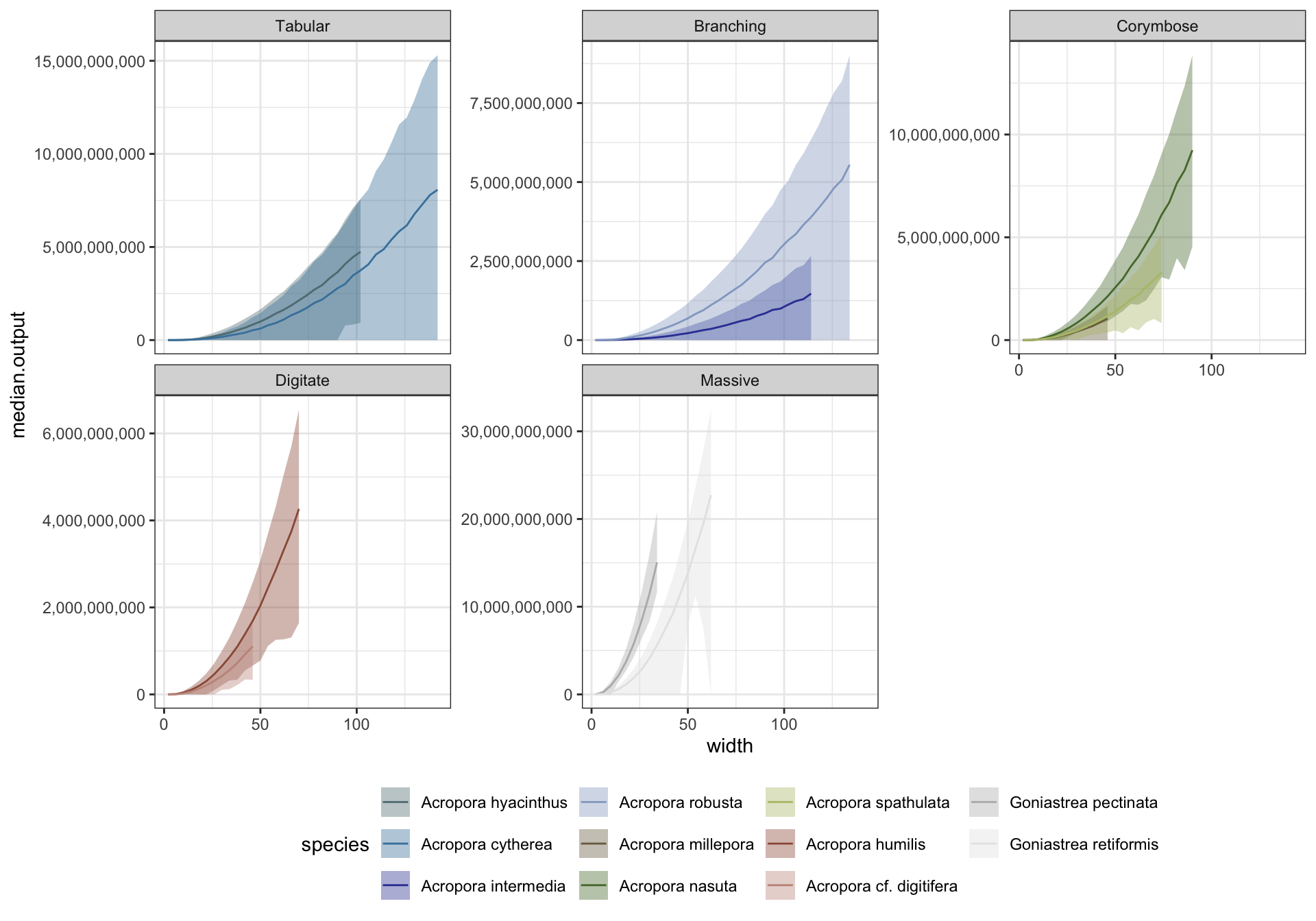
2. Simulate colonies
Combine vars to get total output per colony * species (data.table for predictions for speed):
Code
library(data.table)

# Set number of posterior draws
ndraws <- 5000

# Convert coralsize to data.table
coralsize <- as.data.table(coralsize)

# Step 1: Max width per species
maxwidth_dt <- coralsize[, .(maxwidth = max(width)), by = species]

# Step 2: Build species × width grid
base_newdf <- CJ(
  species = unique(coralsize$species),
  width = seq(2, 200, 4)
)
base_newdf <- merge(base_newdf, maxwidth_dt, by = "species")[width <= maxwidth][, maxwidth := NULL]

# Step 3: Repeat for draws
newdf <- base_newdf[rep(1:.N, each = ndraws)][, draw := rep(1:ndraws, times = .N / ndraws)]

# Step 4: Posterior predictions for each model
pp_polyp   <- posterior_predict(brm_polyp_density, newdata = base_newdf, ndraws = ndraws)
pp_repro   <- posterior_predict(brm_probability, newdata = base_newdf, ndraws = ndraws)
pp_oocytes <- posterior_predict(brm_fecundity, newdata = base_newdf, ndraws = ndraws)

# Step 5: Flatten predictions into long vector
newdf[, polypdensity := as.numeric(pp_polyp)]
newdf[, reproductive_probability := as.numeric(pp_repro)]
newdf[, oocytes := as.numeric(pp_oocytes)]

# Step 6: Sample sterile zone proportions
newdf[, sterile_proportion := sample_sterile_zone(species_vec = species, draw = "random")]

# Step 7: Calculate reproductive output
newdf[, area := pi * (width / 2)^2]
newdf[, colony_polyps := polypdensity * area * 10000]
newdf[, reproductive_polyps := colony_polyps * sterile_proportion]
newdf[, output := reproductive_polyps * oocytes * reproductive_probability]

# Step 8: Summarise posterior output
summary_dt <- newdf[, .(
  median.output = mean(output),
  lower.ci.output = quantile(output, 0.2),
  upper.ci.output = quantile(output, 0.8)
), by = .(species, width)]

# Step 9: Add growthform and factor levels
summary_dt[, species := factor(species, levels = sp_order)]
summary_dt[, growthform := fct_recode(species,
                                      "Tabular"   = "Acropora cytherea",
                                      "Tabular"   = "Acropora hyacinthus",
                                      "Branching" = "Acropora intermedia",
                                      "Branching" = "Acropora robusta",
                                      "Massive"   = "Goniastrea pectinata",
                                      "Massive"   = "Goniastrea retiformis",
                                      "Corymbose" = "Acropora nasuta",
                                      "Corymbose" = "Acropora millepora",
                                      "Corymbose" = "Acropora spathulata",
                                      "Digitate"  = "Acropora cf. digitifera",
                                      "Digitate"  = "Acropora humilis"
)]


ggplot() + theme_bw() +
  geom_line(data=summary_dt, aes(width, median.output, color=species), linewidth=1.2) +
  scale_y_continuous(labels = scales::comma) +
  scale_color_manual(values=sp_pal) + scale_fill_manual(values=sp_pal)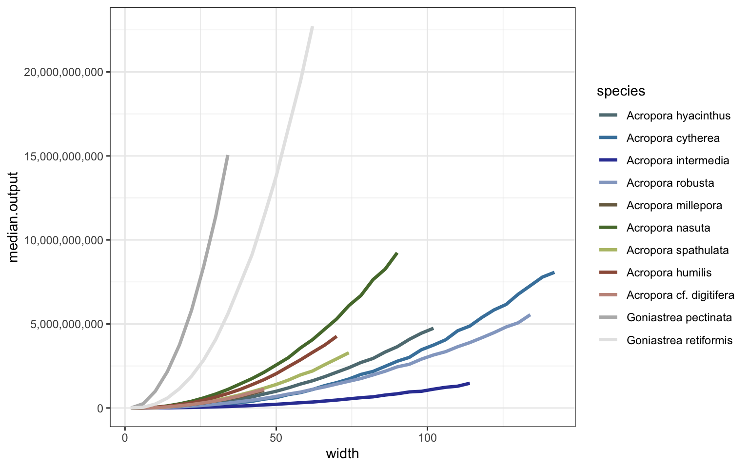
Code
ggplot() +
  theme_bw() +
  facet_wrap(~growthform, scales = "free_y") +
  geom_ribbon(data = summary_dt, aes(width, ymin = lower.ci.output, ymax = upper.ci.output, fill = species), alpha = 0.4) +
  geom_line(data = summary_dt, aes(width, median.output, color = species)) +
  scale_y_continuous(labels = scales::comma) +
  scale_color_manual(values = sp_pal) +
  scale_fill_manual(values = sp_pal) +
  theme(legend.position = "bottom")