allee effects
2024 “bleaching” scenario
simulate 20 X 10m plot at 40% cover:
Code
library(tidyverse)
library(sf)
library(tmap)
library(reefspawn)

seedval = 321

coral_size_2024 <- simulate_coralsize(coralsize |> filter(year==2011),
                                      distribution = "rlnorm",
                                      ndraws = 2000,
                                      seed = seedval)

sf_plot <- setplot(20,10) # default EPSG:3857
coralsizepredictions <- posterior_coral_predict(brm = brm_sizedistribution,
                                                newdata = coral_size_2024,
                                                seed = seedval)

communities <- simulate_community(setplot = sf_plot,
                                  coralcover = 40,
                                  size = coral_size_2024,
                                  seed = seedval)

populations <- simulate_populations(setplot = sf_plot,
                                    size = coral_size_2024,
                                    community = communities,
                                    return="sf",
                                    seed = seedval)


reproductive_populations <- simulate_spawning(populations = populations,
                                        setplot = sf_plot,
                                        seed = 123)


reproductive_populations_postbleaching <- simulate_bleaching(populations = reproductive_populations)


prebleachingplot <- map_populations(setplot = sf_plot,
                populations = reproductive_populations, # or reproductive output, same sf population
                interactive = FALSE) + tm_title("Pre-bleaching")

postbleachingplot <- map_populations(setplot = sf_plot,
                populations = reproductive_populations_postbleaching, # or reproductive output, same sf population
                interactive = FALSE) + tm_title("Post-bleaching")

tmap::tmap_arrange(prebleachingplot, postbleachingplot, ncol=1)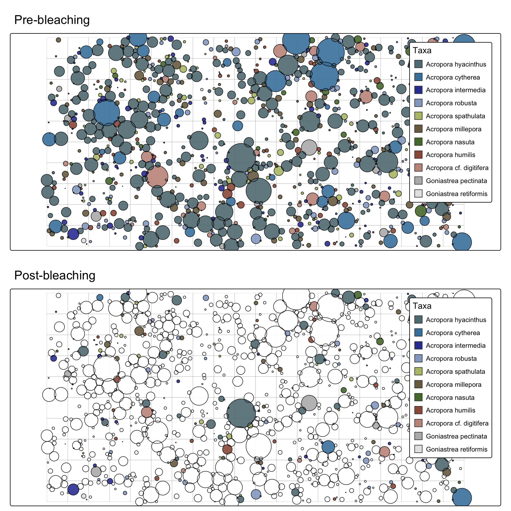
Calculate allee effects (intercolony distances)
Plot intraspecific distance matrix as spatial connectivity (i.e. distances between colonies before and after bleaching in cartesian space)
Code
pre_bleaching_allee <- calculate_allee_effects(populations = reproductive_populations_postbleaching,
                                               metric = "centroid_distance",
                                               label = "pre-bleaching")


post_bleaching_allee <- calculate_allee_effects(populations = reproductive_populations_postbleaching |> filter(status=="unbleached"),
                                                metric = "centroid_distance",
                                                label = "post-bleaching")

all_combined_allee <- rbind(pre_bleaching_allee, post_bleaching_allee) |>
  mutate(status = factor(status, levels=c("pre-bleaching", "post-bleaching")))


tm_shape(all_combined_allee) +
  tm_lines(col="species",
           col.legend = tm_legend_hide(),
           col.scale = tm_scale_categorical(values=sp_pal(), levels.drop=FALSE),
           lwd=0.1) +
  tm_facets_grid(columns="status", rows="species")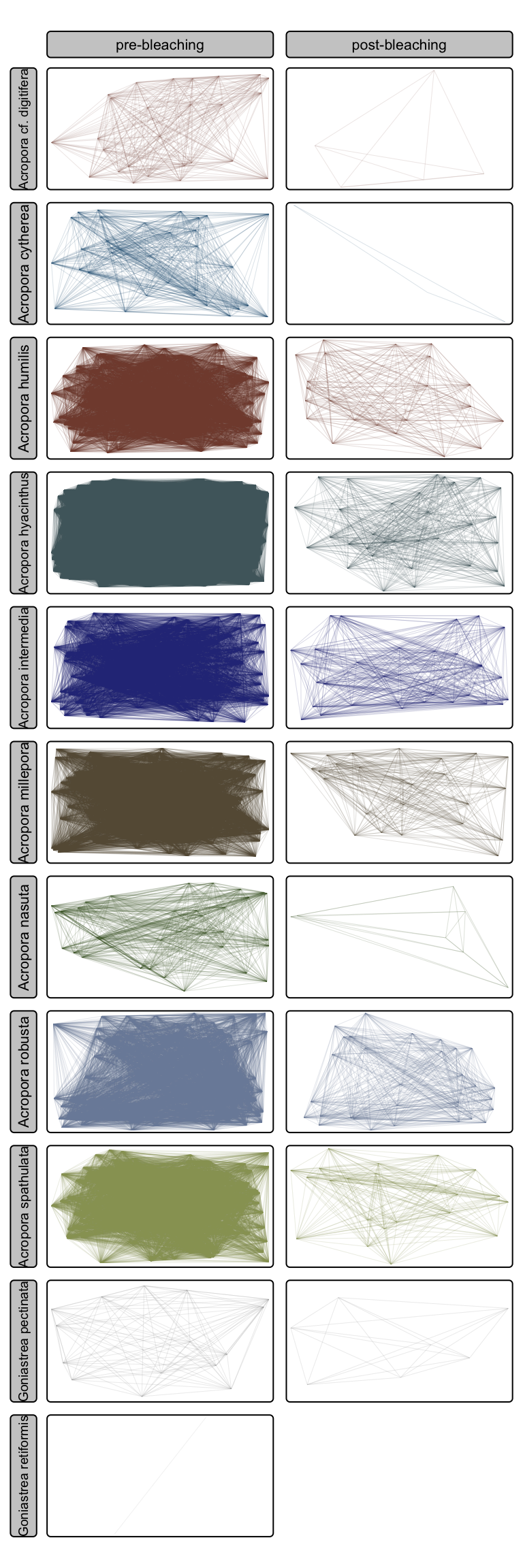
Calculate fertilisation success
Reproduce Fig 2b PNAS paper (check tail for exponential decay later)
Code
# Fit non-linear curve: exponential decay model
library(tidyverse)

# Input data
df <- tibble::tibble(
  distance = c(0, 2, 4, 6, 8, 10, 12, 14, 16, 18, 20),
  fertilization = c(30.1, 23.86, 18.43, 14.23, 10.79, 8.11, 6.07, 4.54, 3.44, 2.46, 1.82)
)

# Exponential decay fit
exp_decay_fit <- nls(
  fertilization ~ a * exp(b * distance) + c,
  data = df,
  start = list(a = 28, b = -0.2, c = 2)
)

# Exponential plateau fit
exp_plateau_fit <- nls(
  fertilization ~ c + a * exp(-b * distance),
  data = df,
  start = list(a = 28, b = 0.2, c = 2)
)

# Generate prediction curves
distance_seq <- seq(0, 30, 0.1)

decay_curve <- tibble(
  distance = distance_seq,
  fertilization = predict(exp_decay_fit, newdata = tibble(distance = distance_seq)),
  model = "Exponential Decay"
)

plateau_curve <- tibble(
  distance = distance_seq,
  fertilization = predict(exp_plateau_fit, newdata = tibble(distance = distance_seq)),
  model = "Exponential Plateau"
)

# Combine curves
curve_df <- bind_rows(decay_curve, plateau_curve)

# Plot
ggplot(df, aes(distance, fertilization)) +
  geom_point(size = 1.2, shape=21) +
  geom_line(data = curve_df, aes(x = distance, y = fertilization, color = model), linewidth = 0.1, show.legend=FALSE) +
  theme_bw() + ylim(0,35) +
  labs(title = "", y = "Fertilization (%)", x = "Intercolony distance (m)")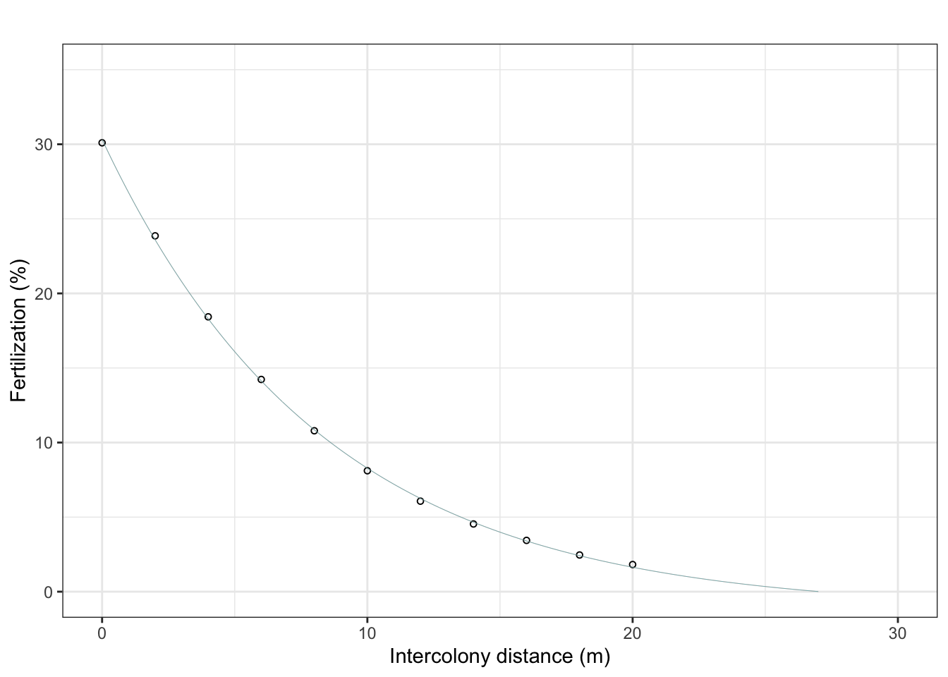
Quantify allee effects (Acropora hyacinthus)
Fit exponential decay to distance data, map fertilisation success (i.e. distance) for a single species- A.hyacinthus
Code
# fit exponential decay to distance data
all_combined_allee_fertilisation <- all_combined_allee |>
   mutate(fertilisation_success = round(predict(exp_decay_fit, newdata = data.frame(distance = centroid_distance)), 2))

allee_hyacinthus <- all_combined_allee_fertilisation |>
  dplyr::filter(species == "Acropora hyacinthus")


tm_shape(allee_hyacinthus) +
  tm_lines(
    col = "fertilisation_success",
    col.scale = tm_scale_continuous(values="brewer.spectral"),
    #col.legend = tm_legend_hide(),
    lwd = 0.1
  ) +
    tm_facets_grid(rows="status") + tm_title("Acropora hyacinthus")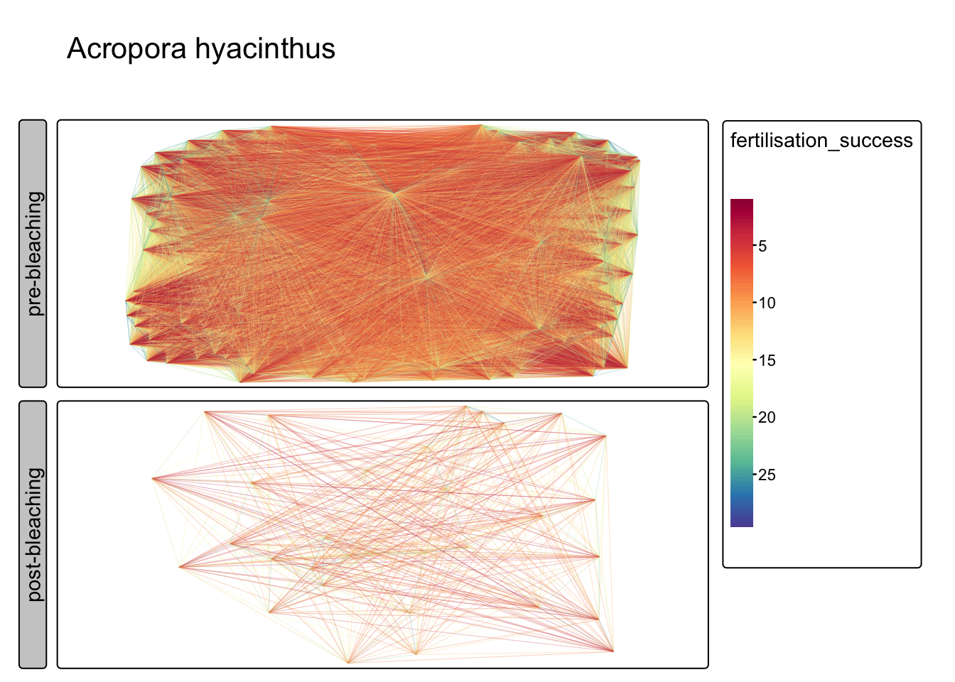
Summary statistics for hyacinthus - 93.6% mortality, 6.7% survival - 180 colonies pre-bleaching, 12 colonies surviving - no clear reduction in intracolony distance (despite mass mortality) - no impact on fertilisation success (assuming homogeneity in dispersal)
Code
a <- reproductive_populations_postbleaching |>
  filter(species == "Acropora hyacinthus") |>
  filter(output > 0) |>
  as.data.frame() |>
  count(status) |>
  mutate(prop = n / sum(n) * 100) |>
  ggplot(aes(x = "", y = prop, fill = status)) +
  geom_col(alpha = 0.3, color = "black", position = "stack", show.legend=FALSE) +
  theme_minimal() +
  ylab("Proportion (%)") +
  xlab("") +
  ggtitle("% mortality pre - post bleaching")  +
    theme(plot.title = element_text(size = 8)) +
  scale_fill_manual(values=c("darksalmon", "darkturquoise"))


b <- reproductive_populations_postbleaching |>
          filter(species=="Acropora hyacinthus") |>
          as.data.frame() |>
          filter(output > 0) |>
          count(status) |>
          mutate(prop = n / sum(n) * 100) |>
   ggplot(aes(x = status, y = n, fill = status)) +
          geom_col(alpha=0.3, col="black", show.legend=FALSE) +
          theme_minimal() +
          ylab("n colonies") +
          xlab("Status") + ggtitle("n colonies per 10*20m2 plot") +
    theme(plot.title = element_text(size = 8)) +
  scale_fill_manual(values=c("darksalmon", "darkturquoise"))


c <- allee_hyacinthus |>
          as.data.frame() |>
          count(status) |>
          mutate(prop = n / sum(n) * 100) |>
          ggplot(aes(x = status, y = n, fill = status)) +
          geom_col(alpha=0.3, col="black", show.legend=FALSE) +
          theme_minimal() +
          ylab("n") +
          xlab("Status") +
          ggtitle("Number of intercolony connections") +
    theme(plot.title = element_text(size = 8)) +
  scale_fill_manual(values=c( "darkturquoise",  "darksalmon"))


  d <-   ggplot() + theme_minimal() + ggtitle("Fertilisation success pre/post bleaching") +
    geom_density(data = allee_hyacinthus,
                 aes(fertilisation_success, color = status, fill = status),
                 alpha = 0.3, show.legend = FALSE)  +
    theme(plot.title = element_text(size = 8)) +
   scale_fill_manual(values=c( "darkturquoise",  "darksalmon")) +
   scale_color_manual(values=c( "darkturquoise",  "darksalmon"))


  e <- ggplot() + theme_minimal() + ggtitle("Inter-colony distance pre/post bleaching") +
    geom_density(data = allee_hyacinthus,
                 aes(centroid_distance, color = status, fill = status), alpha=0.3) +
    theme(plot.title = element_text(size = 8)) +
   scale_fill_manual(values=c( "darkturquoise",  "darksalmon"))+
   scale_color_manual(values=c( "darkturquoise",  "darksalmon"))


  library(patchwork)

  (a+b)/(c+d+e)  + plot_annotation(title = 'Acropora hyacinthus')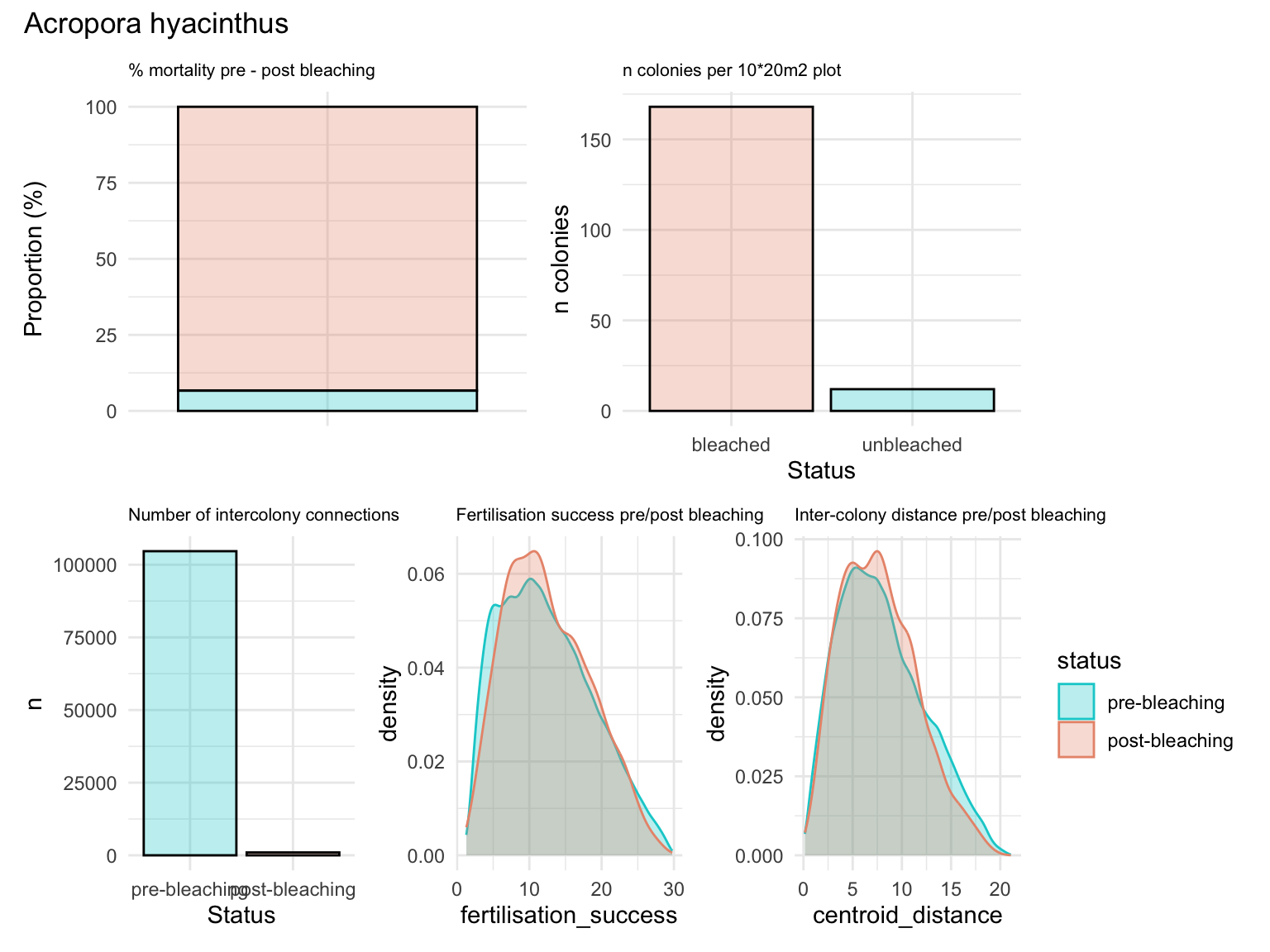
Quantify allee effects (Goniastrea pectinata)
Fit exponential decay to distance data, map fertilisation success (i.e. distance) for a G.pectinata
Code
# fit exponential decay to distance data
all_combined_allee_fertilisation <- all_combined_allee |>
   mutate(fertilisation_success = round(predict(exp_decay_fit, newdata = data.frame(distance = centroid_distance)), 2))

allee_goniastrea <- all_combined_allee_fertilisation |>
  dplyr::filter(species == "Goniastrea pectinata")


tm_shape(allee_goniastrea) +
  tm_lines(
    col = "fertilisation_success",
    col.scale = tm_scale_continuous(values="brewer.spectral"),
    #col.legend = tm_legend_hide(),
    lwd = 0.1
  ) +
    tm_facets_grid(rows="status") + tm_title("Goniastrea pectinata")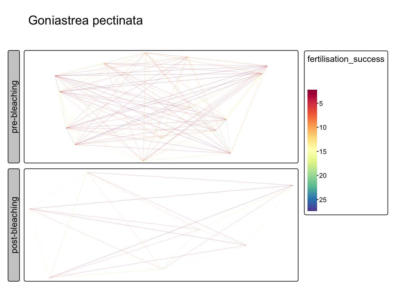
Summary statistics for goniastrea - 93.6% mortality, 6.7% survival - 180 colonies pre-bleaching, 12 colonies surviving - no clear reduction in intracolony distance (despite mass mortality) - no impact on fertilisation success (assuming homogeneity in dispersal)
Code
a <- reproductive_populations_postbleaching |>
  filter(species == "Goniastrea pectinata") |>
  filter(output > 0) |>
  as.data.frame() |>
  count(status) |>
  mutate(prop = n / sum(n) * 100) |>
  ggplot(aes(x = "", y = prop, fill = status)) +
  geom_col(alpha = 0.3, color = "black", position = "stack", show.legend=FALSE) +
  theme_minimal() +
  ylab("Proportion (%)") +
  xlab("") +
  ggtitle("% mortality pre - post bleaching")  +
    theme(plot.title = element_text(size = 8)) +
  scale_fill_manual(values=c("darksalmon", "darkturquoise"))


b <- reproductive_populations_postbleaching |>
          filter(species=="Goniastrea pectinata") |>
          as.data.frame() |>
          filter(output > 0) |>
          count(status) |>
          mutate(prop = n / sum(n) * 100) |>
   ggplot(aes(x = status, y = n, fill = status)) +
          geom_col(alpha=0.3, col="black", show.legend=FALSE) +
          theme_minimal() +
          ylab("n colonies") +
          xlab("Status") + ggtitle("n colonies per 10*20m2 plot") +
    theme(plot.title = element_text(size = 8)) +
  scale_fill_manual(values=c("darksalmon", "darkturquoise"))


c <- allee_goniastrea |>
          as.data.frame() |>
          count(status) |>
          mutate(prop = n / sum(n) * 100) |>
          ggplot(aes(x = status, y = n, fill = status)) +
          geom_col(alpha=0.3, col="black", show.legend=FALSE) +
          theme_minimal() +
          ylab("n") +
          xlab("Status") +
          ggtitle("Number of intercolony connections") +
    theme(plot.title = element_text(size = 8)) +
  scale_fill_manual(values=c( "darkturquoise",  "darksalmon"))


  d <-   ggplot() + theme_minimal() + ggtitle("Fertilisation success pre/post bleaching") +
    geom_density(data = allee_goniastrea,
                 aes(fertilisation_success, color = status, fill = status),
                 alpha = 0.3, show.legend = FALSE)  +
    theme(plot.title = element_text(size = 8)) +
   scale_fill_manual(values=c( "darkturquoise",  "darksalmon")) +
   scale_color_manual(values=c( "darkturquoise",  "darksalmon"))


  e <- ggplot() + theme_minimal() + ggtitle("Inter-colony distance pre/post bleaching") +
    geom_density(data = allee_goniastrea,
                 aes(centroid_distance, color = status, fill = status), alpha=0.3) +
    theme(plot.title = element_text(size = 8)) +
   scale_fill_manual(values=c( "darkturquoise",  "darksalmon"))+
   scale_color_manual(values=c( "darkturquoise",  "darksalmon"))


  library(patchwork)

  (a+b)/(c+d+e) + plot_annotation(title = 'Goniastrea pectinata')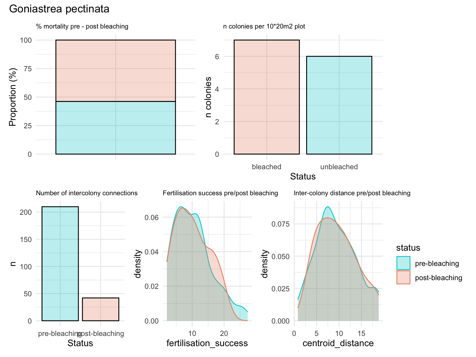
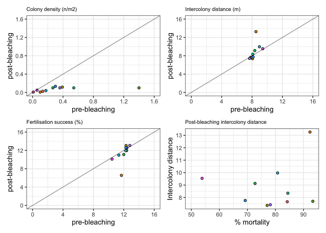
Summary allee effects
Mass reduction in colony densities post-bleaching, yet minimal reduction in intercolony distance / fertilisation success No impact as low as 0.5 colonies per m2 (but will impact rare taxa (either post-bleaching losses below a threshold or initially rare species)
Code
tmp <- reproductive_populations_postbleaching |>
  filter(output > 0) |>
  as.data.frame() |>
  count(species, status) |>
  mutate(n = n / 120) |>
  pivot_wider(names_from="status", values_from="n") |>
  mutate(prop = bleached/(bleached+unbleached)  * 100)

allee1 <- ggplot() + theme_bw() +
  geom_point(data = tmp, aes(bleached, unbleached, fill=species), shape=21, size=1.5, show.legend=FALSE) +
#  ggrepel::geom_text_repel(data = tmp, aes(bleached, unbleached, label=species), max.overlaps=100) +
  scale_x_continuous(limits=c(0,1.6), breaks = seq(0,1.6,0.4)) +
  scale_y_continuous(limits=c(0,1.6), breaks = seq(0,1.6,0.4)) +
  geom_abline(alpha=0.4) +
  xlab("pre-bleaching") +
  ylab("post-bleaching") +
  ggtitle("Colony density (n/m2)") +
  theme(plot.title = element_text(size = 8))


tmp2 <- all_combined_allee_fertilisation |>
  as.data.frame() |>
  select(species, status, centroid_distance) |>
  group_by(species, status) |>
  summarise(distance = mean(centroid_distance)) |>
  pivot_wider(names_from="status", values_from="distance") |>
  rename(pre_bleaching = 2, post_bleaching =3)


allee2 <- ggplot() + theme_bw() +
  geom_point(data = tmp2, aes(pre_bleaching, post_bleaching, fill=species), shape=21, size=1.5, show.legend=FALSE) +
#  ggrepel::geom_text_repel(data = tmp, aes(bleached, unbleached, label=species), max.overlaps=100) +
  scale_x_continuous(limits=c(0,16), breaks = seq(0,16,4)) +
  scale_y_continuous(limits=c(0,16), breaks = seq(0,16,4)) +
  geom_abline(alpha=0.4) +
  xlab("pre-bleaching") +
  ylab("post-bleaching") +
  ggtitle("Intercolony distance (m)") +
  theme(plot.title = element_text(size = 8))


tmp3 <- all_combined_allee_fertilisation |>
  as.data.frame() |>
  select(species, status, fertilisation_success) |>
  group_by(species, status) |>
  summarise(distance = mean(fertilisation_success)) |>
  pivot_wider(names_from="status", values_from="distance") |>
  rename(pre_bleaching = 2, post_bleaching =3)


allee3 <- ggplot() + theme_bw() +
  geom_point(data = tmp3, aes(pre_bleaching, post_bleaching, fill=species), shape=21, size=1.5, show.legend=FALSE) +
#  ggrepel::geom_text_repel(data = tmp, aes(bleached, unbleached, label=species), max.overlaps=100) +
  scale_x_continuous(limits=c(0,16), breaks = seq(0,16,4)) +
  scale_y_continuous(limits=c(0,16), breaks = seq(0,16,4)) +
  geom_abline(alpha=0.4) +
  xlab("pre-bleaching") +
  ylab("post-bleaching") +
  ggtitle("Fertilisation success (%)") +
  theme(plot.title = element_text(size = 8))


summary_allee <- left_join(tmp, tmp2)


allee4 <- ggplot() + theme_bw() +
  geom_point(data = summary_allee, aes(prop, post_bleaching, fill=species), shape=21, size=1.5, show.legend=FALSE) +
#  ggrepel::geom_text_repel(data = tmp, aes(bleached, unbleached, label=species), max.overlaps=100) +
  geom_abline(alpha=0.4) +
  xlab("% mortality")+
  ylab("Intercolony distance") +
  ggtitle("Post-bleaching intercolony distance") +
  theme(plot.title = element_text(size = 8))

(allee1 + allee2) / (allee3 + allee4)