Detecting long-term shifts in annual SST-SSTA-DHW data using the reconstructed historical OISST2 dataset using BEAST (a Bayesian model averaging algorithm) to detect abrupt changes, trends, and periodic variations.
Sea Surface Temperatures
GBR-wide mean summer SST annual time series (°C):
- Calculate spatial mean (GBR-area mean SST for each day)
- Filter Jan–Mar (peak austral-summer conditions for the GBR).
- Aggregate for each year the mean of the Jan–Mar daily GBR-area means
Output:
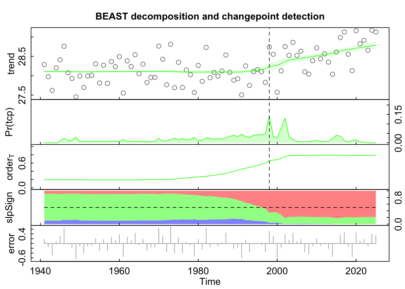
- Top (trend): grey dots are annual Jan–Mar SST metric; green line is BEAST’s estimated underlying trend, flat to slightly variable through mid-century, then shows a clear upward shift / acceleration beginning around the late 1990s into early 2000s, continuing upward thereafter.
- Pr(tcp): this is the posterior probability of a trend changepoint at each year. The dominant peak is around ~1998–2002, meaning BEAST sees the most plausible structural change in the long-term evolution there (often interpreted as a regime shift / onset of sustained warming in this metric).
- orderT: BEAST’s inferred trend complexity/order over time (how curved the trend is allowed/needed to be). orderT rises into the late 1990s/early 2000s and then stabilizes higher, consistent with the trend needing more structure once the warming period begins (i.e., not just noise around a flat baseline).
- slpSign: posterior support for the sign of the trend slope through time. Pre-~1998 it’s closer to “weak/uncertain or mixed,” then post-~1998 it shifts strongly toward persistent positive slope (sustained warming) for the remainder of the record.
- error: residuals (what’s left after removing the fitted components), i.e. interannual variability around the inferred trend.
Code
library(terra)
library(Rbeast)
library(tidyverse)

GBR_OISST2_SST <- rast("/Users/rof011/GBR-dhw/datasets/GBR_OISST2_SST.tif")

sst_ts <- terra::global(GBR_OISST2_SST, mean, na.rm = TRUE) %>%
  mutate(date = as.Date(rownames(.))) |>
  mutate(
    year  = year(date),
    month = month(date),
    austral_year = if_else(month == 12L, year + 1L, year)  # Dec belongs to next year
  ) %>%
  filter(month %in% seq(1:3)) %>%
  filter(austral_year > 1940, austral_year < 2026) %>%
  group_by(austral_year) %>%
  summarise(sst = mean(mean, na.rm = TRUE), .groups = "drop") %>%
  rename(year = austral_year)

sst_ts <- sst_ts %>% arrange(year)
y_sst <- sst_ts$sst
t_sst <- sst_ts$year

beast_sst <- beast(
  y_sst,
  start  = t_sst[1],
  deltat = 1,
  season = "none",
  print.progress = FALSE,
  quiet = TRUE
)

cp_sst   <- beast_sst$trend$cp
cppr_sst <- beast_sst$trend$cpPr
if (is.null(cppr_sst)) cppr_sst <- beast_sst$trend$cpProb

sst_cp_tbl <- tibble(cp = cp_sst, cp_prob = cppr_sst) %>%
  mutate(year = as.integer(round(cp))) %>%
  arrange(desc(cp_prob))

breakpoints_sst <- sst_cp_tbl$cp[1:min(2, nrow(sst_cp_tbl))]
breakyears_sst  <- sst_cp_tbl$year[1:min(2, nrow(sst_cp_tbl))]

plot(beast_sst)
SST Anomalies
GBR-wide mean summer SSTA annual time series (°C anomaly):
- Calculate spatial mean (GBR-area mean SST anomaly for each day)
- Filter Jan–Mar (peak austral-summer conditions for the GBR).
- Aggregate for each year the mean of the Jan–Mar daily GBR-area means
Output:
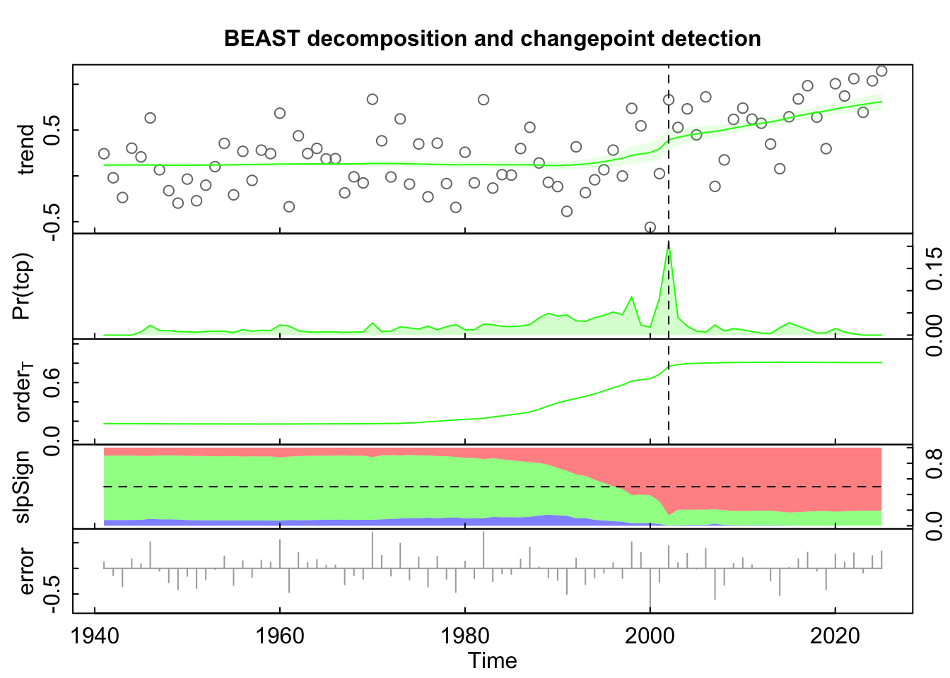
- Trend: near-flat to mildly variable through mid-century, then shows a clear upward shift / acceleration beginning around the late 1990s into early 2000s, continuing upward thereafter.
- Pr(tcp): dominant peak is around ~2000–2002, meaning BEAST sees the most plausible structural change in the long-term evolution there (often interpreted as a regime shift / onset of sustained positive anomalies in this metric).
- orderT: rises into the late 1990s/early 2000s and then stabilizes higher, consistent with the trend needing more structure once the anomaly regime begins (i.e., not just noise around ~0).
- slpSign: Pre-~2000 closer to “weak/uncertain or mixed,” then post-~2000 it shifts strongly toward persistent positive slope (sustained warming anomalies) for the remainder of the record.
Code
GBR_OISST2_SSTA <- rast("/Users/rof011/GBR-dhw/datasets/GBR_OISST2_SSTA.tif")

ssta_ts <- terra::global(GBR_OISST2_SSTA, mean, na.rm = TRUE) %>%
  mutate(date = as.Date(rownames(.))) |>
  mutate(
    year  = year(date),
    month = month(date),
    austral_year = if_else(month == 12L, year + 1L, year)  # Dec belongs to next year
  ) %>%
  filter(month %in% c(12, 1, 2, 3)) %>%
  filter(austral_year > 1940, austral_year < 2026) %>%
  group_by(austral_year) %>%
  summarise(ssta = mean(mean, na.rm = TRUE), .groups = "drop") %>%
  rename(year = austral_year)


ssta_ts <- ssta_ts %>% arrange(year)
y_ssta <- ssta_ts$ssta
t_ssta <- ssta_ts$year

beast_ssta <- beast(
  y_ssta,
  start  = t_ssta[1],
  deltat = 1,
  season = "none",
  print.progress = FALSE,
  quiet = TRUE
)

cp_ssta   <- beast_ssta$trend$cp
cppr_ssta <- beast_ssta$trend$cpPr
if (is.null(cppr_ssta)) cppr_ssta <- beast_ssta$trend$cpProb

ssta_cp_tbl <- tibble(cp = cp_ssta, cp_prob = cppr_ssta) %>%
  mutate(year = as.integer(round(cp))) %>%
  arrange(desc(cp_prob))

breakpoints_ssta <- ssta_cp_tbl$cp[1:min(2, nrow(ssta_cp_tbl))]
breakyears_ssta  <- ssta_cp_tbl$year[1:min(2, nrow(ssta_cp_tbl))]

plot(beast_ssta)
Degree Heating Weeks
GBR-wide peak heat stress (DHW) austral-year annual time series (°C-weeks):
- Calculate spatial mean (GBR-area mean DHW for each day)
- Aggregate for each year the maximum of the daily GBR-area mean DHW values
Output:
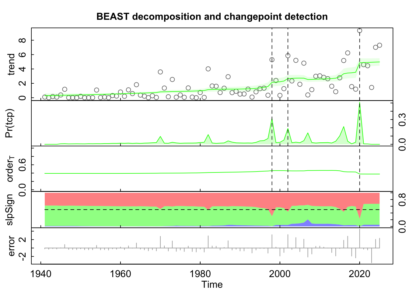
- Top (trend): low/near-zero through mid-century, then rising with clear step-like increases around the late 1990s–early 2000s and another strong increase around ~2020, indicating higher typical peak heat-stress years in the recent period.
- Pr(tcp): prominent peaks occur around ~1998–2002 and a very strong peak around ~2020, meaning BEAST sees major structural changes in the long-term evolution of peak heat stress at those times (often interpreted as shifts to higher heat-stress regimes and/or increased frequency of extreme DHW years).
- orderT: fairly stable for most of the record, with a change around the most recent breakpoint, consistent with the trend structure being dominated by a few step/acceleration periods rather than many small bends.
- slpSign: distribution is dominated by positive-slope support across most of the record, with localized dips around breakpoint windows, consistent with an overall increasing trajectory in peak DHW despite substantial year-to-year variability.
- error: larger excursions in recent decades reflecting more extreme departures in peak DHW years.
Code
GBR_OISST2_DHW <- rast("/Users/rof011/GBR-dhw/datasets/GBR_OISST2_DHW.tif")

sst_dhw <- terra::global(GBR_OISST2_DHW, mean, na.rm = TRUE) %>%
  mutate(date = as.Date(rownames(.))) |>
  mutate(
    year  = year(date),
    month = month(date),
    austral_year = if_else(month == 12L, year + 1L, year)  # Dec belongs to next year
  ) %>%
  #filter(month %in% c(12, 1, 2, 3)) %>%
  filter(austral_year > 1940, austral_year < 2026) %>%
  group_by(austral_year) %>%
  summarise(dhw = max(mean, na.rm = TRUE), .groups = "drop") %>%
  rename(year = austral_year)


sst_dhw <- sst_dhw %>% arrange(year)
y_dhw <- sst_dhw$dhw
t_dhw <- sst_dhw$year

beast_dhw <- beast(
  y_dhw,
  start  = t_dhw[1],
  deltat = 1,
  season = "none",
  print.progress = FALSE,
  quiet = TRUE
)

cp_dhw   <- beast_dhw$trend$cp
cppr_dhw <- beast_dhw$trend$cpPr
if (is.null(cppr_dhw)) cppr_dhw <- beast_dhw$trend$cpProb

sst_cp_tbl <- tibble(cp = cp_dhw, cp_prob = cppr_dhw) %>%
  mutate(year = as.integer(round(cp))) %>%
  arrange(desc(cp_prob))

breakpoints_dhw <- sst_cp_tbl$cp[1:min(2, nrow(sst_cp_tbl))]
breakyears_dhw  <- sst_cp_tbl$year[1:min(2, nrow(sst_cp_tbl))]

plot(beast_dhw)