2024 mass coral bleaching event: methods
George Roff
2024-03-29
Below is an intiial analysis of the DHW from the 2024 mass coral bleaching event on the Great Barrier Reef.
i) Great Barrier Reef shp file
First, load the GBRMPA shp files for the Great Barrier Reef. For reproducibility the files are downloadable from Bozec et al 2022, and may differ from the official GBRMPA files available from the GBRMPA geoportal.
library(httr)
library(tidyverse)
library(janitor)
library(sf)
library(stars)
library(raster)
library(exactextractr)
library(tmap)
library(kableExtra)
library(reactable)
library(ggplot2)
library(terra)
library(tidyterra)

# write a function to get GBR shape file boundaries from eAtlas
get_gbr_shape <- function(crs="EPSG:20353", source="file"){

  if (source=="url"){
    #download from eAtlas
    url <- "https://nextcloud.eatlas.org.au/s/xQ8neGxxCbgWGSd/download/TS_AIMS_NESP_Torres_Strait_Features_V1b_with_GBR_Features.zip"
    destfile <- "TS_AIMS_NESP_Torres_Strait_Features_V1b_with_GBR_Features.zip"
    GET(url, write_disk(destfile, overwrite = TRUE))
    if (!dir.exists("unzipped_files")) {
      dir.create("unzipped_files")
    }
    unzip("TS_AIMS_NESP_Torres_Strait_Features_V1b_with_GBR_Features.zip", exdir = "unzipped_files")
    shapefile_path <- "unzipped_files/TS_AIMS_NESP_Torres_Strait_Features_V1b_with_GBR_Features.shp"

    gbr_shape <- st_read(shapefile_path, quiet=TRUE) %>%
      mutate(longitude = st_drop_geometry(.)$X_COORD,
             latitude = st_drop_geometry(.)$Y_COORD) |>
      filter(FEAT_NAME=="Reef") |>
      st_set_crs(4283) |>
      st_transform(20353) |>
      st_make_valid() |>
      clean_names() |>
      dplyr::select(loc_name_s, qld_name, gbr_name, label_id, geometry, longitude, latitude) |>
      mutate(gbr_name = as.factor(gbr_name)) |>
      mutate(label_id = as.factor(label_id))

    zones <- read.csv("/Users/rof011/GBR-coral-bleaching/data/gbr_zones.csv")

    gbr_shape_output <- left_join(gbr_shape, zones, by="label_id")

    return(gbr_shape)

  } else if (source=="file"){
   #read from disk
   shapefile_path <- "/Users/rof011/GBR-coral-bleaching/data/Great_Barrier_Reef_Features.shp"

    gbr_shape <- st_read(shapefile_path, quiet=TRUE) %>%
      mutate(longitude = st_drop_geometry(.)$X_COORD,
             latitude = st_drop_geometry(.)$Y_COORD) |>
      filter(FEAT_NAME=="Reef") |>
      st_set_crs(4283) |>
      st_transform(20353) |>
      st_make_valid() |>
      clean_names() |>
      dplyr::select(loc_name_s, qld_name, gbr_name, label_id, geometry, longitude, latitude,
             area_ha) |>
      mutate(gbr_name = as.factor(gbr_name)) |>
      mutate(label_id = as.factor(label_id))

    zones <- read.csv("/Users/rof011/GBR-coral-bleaching/data/gbr_zones.csv")

    gbr_shape_output <- left_join(gbr_shape, zones, by="label_id")

    return(gbr_shape)
  }

}


### note that sf throws topology errors:
# Error in scan(text = lst[[length(lst)]], quiet = TRUE) :
#   scan() expected 'a real', got 'TopologyException:'
# Error in (function (msg)  :
#   TopologyException: CoverageUnion cannot process incorrectly noded inputs.


gbr_shape <- get_gbr_shape(source="file") |>
  mutate(id=sub("([a-zA-Z])$", "", label_id)) |> # drop multi-named sub-reef ID
  group_by(gbr_name, id) |>
  summarise() |>
  st_make_valid()

# get distinct label_ID for each reef without sub-headings
# complex as some reefs (e.g. U/N) are catch-all "unknown reefs"
gbr_shape_label_ID <- get_gbr_shape() |>
  as_tibble() |>
  mutate(gbr_name=as.factor(gbr_name)) |>
  mutate(id=sub("([a-zA-Z])$", "", label_id)) |>
  dplyr::select(gbr_name, id) |>
  distinct(gbr_name,id)

### this approach seems to give the same approx reef area as the raw data:
gbr_shape_raw <- get_gbr_shape()
# gbr_shape |> st_area() |> sum()      # 28560112188 [m^2]
# gbr_shape_raw |> st_area() |> sum()  # 28560118763 [m^2]


head(gbr_shape) |> kable("html") %>%
  kable_styling("striped", font_size=11) %>%
scroll_box(width = "100%")| gbr_name | id | geometry |
|---|---|---|
| (Big) Broadhurst Reef (No 1) | 18-100 | POLYGON ((1848551 7867941, … |
| (Big) Broadhurst Reef (No 2) | 18-100 | POLYGON ((1845249 7862813, … |
| (Big) Stevens Reef | 20-295 | POLYGON ((2094621 7653332, … |
| (Little) Broadhurst Reef | 18-106 | POLYGON ((1846710 7851185, … |
| (Little) Stevens Reef | 20-294 | POLYGON ((2085467 7656254, … |
| Abott Reef | 19-222 | POLYGON ((2119752 7720364, … |
There are 3724 reefs, with seperate polygons for each reef label
identifier (e.g. U/N Reef has 09-361a through to 09-361f). Individual
polygons per reef ID were merged with sf::union to form
multipolygons (see example for U/N 20-299 reef which has 9 separate
label_id components).
tmap_mode("plot")

a <- tm_shape(gbr_shape_raw |> filter(grepl("20-299", label_id))) +
  tm_polygons("loc_name_s", legend.show=FALSE) +
  tm_graticules() +
  tm_layout(main.title="U/N Reef (20-299) ", main.title.position = "center", main.title.size = 1) +
  tmap_options(max.categories = 57)

b <- tm_shape(gbr_shape  |> filter(grepl("20-299", id))) +
  tm_polygons("aquamarine4", alpha=0.2) +
  tm_layout(main.title="U/N Reef (20-299) merged", main.title.position = "center", main.title.size = 1) +
   tm_graticules()

tmap_arrange(a,b, ncol=2)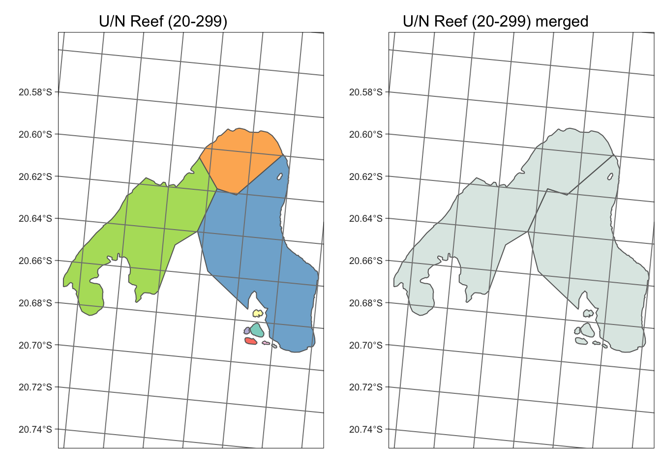
ii) NOAA CRW DHW data
The NOAA Coral Reef Watch (CRW) daily global 5km satellite coral bleaching Degree Heating Week (DHW) is a metric that shows accumulated heat stress.
- “There is a risk of coral bleaching when the DHW value reaches 4 °C-weeks. By the time the DHW value reaches 8 °C-weeks, reef-wide coral bleaching with mortality of heat-sensitive corals is likely. If the accumulated heat stress continues to build further and exceeds a DHW value of 12 °C-weeks, multi-species mortality becomes likely”
The data is available from 01/04/1984 to present day (with a ~2 day lag for processing). Data was extracted for cells within the GBR boundaries as determined by the boundary box (plus a 1km buffer) from the GBR shape file above. Daily DHW were extracted for all 38 years (1985-2023) between 1st January to 1st July, on the assumption that the maximum heatstress would have passed by Austral winter (01/07) in each year.
For each gridcell, the maximum DHW value per year (“yearly maximum DHW”, Van Hooidonk & Huber 2009) was extracted for each year (1986:2024). DHW for 2024 were extracted separately due to an incomplete timeseries at the time of analysis. The approaches to calculating DHW on the GBR differ among studies, for example:
- “For 1998, 2002 and 2020, we used the maximum DHW for each year because bleaching was recorded after the peak. In 2016 and 2017, when bleaching was recorded prior to the maximum DHW for those years, we used the accumulated DHW on the date when bleaching was observed” - Hughes et al. (2020) Current Biology
Further analysis on the distribution/shape of DHW will inform how the 2024 event compares to previous in terms of thermal profiles, but for an initial analysis on DHW the simple approach here uses yearly maximum DHW.
Note: each year of data is ~480mb in size, so total download size is ~15gb and may take some time
gbr_shape_bbox <- gbr_shape |>
  st_transform(4326) |>
  st_bbox()
gbr_shape_bbox <- gbr_shape |>
  st_transform(4326) |>
  st_bbox() |>
  st_as_sfc() |>
  st_buffer(1) |>
  st_bbox()

# custom function for DHW conversion to spatraster
# (there are better functions to download erdapp data e.g. rerddap::griddap but this works for spatraster conversion ofyearly maximum DHW per polygon)
get_dhw_gbr <- function(timestart, timeend, timeout = 60, crs = "EPSG:20353") {
  gbr_dhw_url <- paste0(
    "https://coastwatch.pfeg.noaa.gov/erddap/griddap/NOAA_DHW.csv?", "CRW_DHW", "%5B(", timestart,
    "T12:00:00Z):1:(", timeend, "T12:00:00Z)%5D%5B(",
    -24.86075, "):1:(", -10.27304, ")%5D%5B(",
    141.9369, "):1:(", 153.2032,
    ")%5D"
  )
  temp_file <- tempfile(fileext = ".csv")
  GET(url = gbr_dhw_url, write_disk(temp_file, overwrite = TRUE), timeout(timeout))
  csvdata <- read.csv(temp_file, header = TRUE, skip = 1)
  write_csv(csvdata, paste0("dhw_", start_date, "_raw.csv"))
  print(paste0("Downloading ", start_date, " - ", end_date))
  csvdata <- csvdata |>
    dplyr::select(2, 3, 4) |>
    dplyr::group_by(degrees_east, degrees_north) |>
    summarise(dhw = max(Celsius.weeks))
  gbr_dhw <- tidyterra::as_spatraster(csvdata, crs = "EPSG:4326") |> project("EPSG:20353")
  return(gbr_dhw)
}

# Loop the function across years from 1981 to 2023

gbr_dhw_data <- list()

for (year in 1985:2023) {
  start_date <- paste0(year, "-01-01") # Define start and end dates for the given year
  end_date <- paste0(year, "-07-01")
  dhw_data <- tryCatch(
    { # Fetch the DHW data for the GBR
      get_dhw_gbr(start_date, end_date, timeout = 500)
    },
    error = function(e) { # Use tryCatch to handle  errors or timeouts
      message(paste("Error fetching data for year", year, ":", e$message))
      NULL # Return NULL if there was an error
    }
  )

  gbr_dhw_data[[as.character(year)]] <- dhw_data # Store the list using the year as the name
}

# Ammend 2024 data

for (year in 2024) {
  start_date <- paste0(year, "-01-01") # Define start and end dates for the given year
  end_date <- paste0(year, "-07-01")
  dhw_data <- tryCatch(
    { # Fetch the DHW data for the GBR
      get_dhw_gbr(start_date, end_date, timeout = 500)
    },
    error = function(e) { # Use tryCatch to handle  errors or timeouts
      message(paste("Error fetching data for year", year, ":", e$message))
      NULL # Return NULL if there was an error
    }
  )

  gbr_dhw_data[[as.character(year)]] <- dhw_data # Store the list using the year as the name
}


# function borrowed from FAMEFMR::saveSpatRasterList:
gbr_dhw_data_list <- rapply(gbr_dhw_data_list, f = terra::wrap, classes = "SpatRaster", how = "replace")
qs::qsave(gbr_dhw_data_list, "gbr_dhw_data.RData")
iii) Spatial calculations
As DHW is automatically calculated each day in the NOAA dataset, the
years in max DHW refer to the year of bleaching (e.g. 2016 = cumulative
heatstress from the end of 2015 and the start of 2016). For each reef
multipolygon in the gbr_shape dataset, the mean yearly
maximum DHW in each year was calculated using an area-weighted approach.
exactextractr::exact_extract was used over
stars::st_extract, vect::extract, and
raster::extract due to performance
issues with
stars/terra/rast.
The exact_extract approach used below is conservative in
that for larger reef polygons (or multipolygons) the function calculates
the mean value of cells that intersect the polygon,
weighted by the fraction cell coverage (as opposed to taking the
max value across all underlying cells). Undefined (NA)
values are ignored when they occur in the value raster, and cause the
output to be NA when present in the weights (check these later in the
inshore reefs). Below is a summary of the output:
library(reactable)

gbr_shape_dhw_list <- qs::qread("/Users/rof011/GBR-coral-bleaching/data/gbr_dhw_data.RData")
gbr_shape_dhw_list <- lapply(gbr_shape_dhw_list, function(x) terra::unwrap(x))
gbr_shape_dhw_list <- terra::rast(gbr_shape_dhw_list)
names(gbr_shape_dhw_list) <- paste0("year_", seq(1986, 2024, 1))

year_list <- paste0("year_", seq(1986, 2024, 1))
gbr_shape_dhw <- gbr_shape

for (i in year_list) {
  year_col_name <- paste("dhw_max", sub("^.*_", "", i), sep = "_")
  gbr_shape_dhw[[year_col_name]] <- exact_extract(gbr_shape_dhw_list[[i]],
    progress = FALSE,
    gbr_shape_dhw, fun = "mean", weights = "area"
  )
}


head(gbr_shape_dhw) |>
  kable("html") |>
  kable_styling("striped", font_size = 11) |>
scroll_box(width = "100%")| gbr_name | id | geometry | dhw_max_1986 | dhw_max_1987 | dhw_max_1988 | dhw_max_1989 | dhw_max_1990 | dhw_max_1991 | dhw_max_1992 | dhw_max_1993 | dhw_max_1994 | dhw_max_1995 | dhw_max_1996 | dhw_max_1997 | dhw_max_1998 | dhw_max_1999 | dhw_max_2000 | dhw_max_2001 | dhw_max_2002 | dhw_max_2003 | dhw_max_2004 | dhw_max_2005 | dhw_max_2006 | dhw_max_2007 | dhw_max_2008 | dhw_max_2009 | dhw_max_2010 | dhw_max_2011 | dhw_max_2012 | dhw_max_2013 | dhw_max_2014 | dhw_max_2015 | dhw_max_2016 | dhw_max_2017 | dhw_max_2018 | dhw_max_2019 | dhw_max_2020 | dhw_max_2021 | dhw_max_2022 | dhw_max_2023 | dhw_max_2024 |
|---|---|---|---|---|---|---|---|---|---|---|---|---|---|---|---|---|---|---|---|---|---|---|---|---|---|---|---|---|---|---|---|---|---|---|---|---|---|---|---|---|---|
| (Big) Broadhurst Reef (No 1) | 18-100 | POLYGON ((1848551 7867941, … | 0.4779795 | 6.827402 | 0.000000 | 0.1597545 | 0.7435788 | 0.0000000 | 0.000000 | 0 | 1.7756083 | 1.6970549 | 0.4418001 | 0 | 0.3921288 | 0.4099048 | 0 | 0.6378967 | 2.2812221 | 0 | 2.099609 | 0.6406564 | 0.0000000 | 0 | 0.0000000 | 0.0086903 | 0.6626197 | 0.2797973 | 0.8909236 | 0.9841175 | 0 | 1.9966893 | 2.639892 | 3.855308 | 0.0000000 | 0 | 4.845179 | 0 | 5.318794 | 1.0536289 | 3.319114 |
| (Big) Broadhurst Reef (No 2) | 18-100 | POLYGON ((1845249 7862813, … | 0.4809034 | 6.690235 | 0.000000 | 0.1626551 | 0.7322140 | 0.0000000 | 0.000000 | 0 | 1.8063999 | 1.7350723 | 0.3083107 | 0 | 0.2800516 | 0.4745746 | 0 | 0.5255354 | 1.9665437 | 0 | 2.207775 | 0.5768712 | 0.0000000 | 0 | 0.0000000 | 0.0397638 | 0.6499974 | 0.5694084 | 0.9334313 | 1.0662649 | 0 | 1.9251226 | 2.608260 | 3.985060 | 0.0000000 | 0 | 4.911906 | 0 | 5.216156 | 1.0033153 | 3.714746 |
| (Big) Stevens Reef | 20-295 | POLYGON ((2094621 7653332, … | 2.2126808 | 7.462231 | 0.000000 | 0.0000000 | 0.6870964 | 0.3540293 | 1.372475 | 0 | 0.0930394 | 1.1178683 | 0.0926058 | 0 | 1.7353671 | 0.1865064 | 0 | 0.0013572 | 7.0890689 | 0 | 4.832458 | 0.2291969 | 1.4887915 | 0 | 0.6001107 | 0.8347213 | 2.2275841 | 0.0000000 | 0.7364363 | 0.6408299 | 0 | 1.2891974 | 1.597199 | 4.002799 | 0.0894790 | 0 | 8.630629 | 0 | 5.692474 | 0.8342787 | 8.230654 |
| (Little) Broadhurst Reef | 18-106 | POLYGON ((1846710 7851185, … | 0.4927949 | 7.060939 | 0.000000 | 0.1851825 | 0.7358017 | 0.0000000 | 0.000000 | 0 | 1.7554580 | 1.9170403 | 0.6352469 | 0 | 1.0039911 | 0.5008817 | 0 | 0.5964878 | 2.9083798 | 0 | 2.061579 | 1.0029445 | 0.0133093 | 0 | 0.0000000 | 0.0000000 | 0.7555013 | 0.2112552 | 0.8949642 | 1.1583098 | 0 | 2.1319892 | 2.261860 | 4.152460 | 0.0000000 | 0 | 4.817797 | 0 | 5.554096 | 1.2604388 | 3.465622 |
| (Little) Stevens Reef | 20-294 | POLYGON ((2085467 7656254, … | 2.1869435 | 7.334218 | 0.000000 | 0.0000000 | 0.7461356 | 0.6261856 | 1.198692 | 0 | 0.0085639 | 0.9957811 | 0.1803312 | 0 | 1.9897678 | 0.2502062 | 0 | 0.0000000 | 6.7362270 | 0 | 4.782020 | 0.3121046 | 1.6231992 | 0 | 0.4489488 | 0.9118187 | 2.2421041 | 0.0000000 | 0.8632997 | 0.6447247 | 0 | 1.2262332 | 1.900885 | 3.752129 | 0.1179417 | 0 | 9.029800 | 0 | 6.001618 | 1.0063132 | 8.097749 |
| Abott Reef | 19-222 | POLYGON ((2119752 7720364, … | 0.7593529 | 5.319762 | 0.594146 | 0.1600000 | 0.3113776 | 0.0000000 | 0.000000 | 0 | 0.1686566 | 0.7345553 | 0.1500000 | 0 | 1.1293507 | 0.0000000 | 0 | 1.1302553 | 0.9077468 | 0 | 3.292808 | 0.1700677 | 0.4479577 | 0 | 0.3000000 | 2.9156933 | 0.7369853 | 0.4514952 | 0.4714453 | 0.0000000 | 0 | 0.4719019 | 2.083957 | 2.504015 | 0.0000000 | 0 | 4.460752 | 0 | 4.484212 | 0.6828330 | 9.708863 |
saveRDS(gbr_shape_dhw, "/Users/rof011/GBR-coral-bleaching/data/gbr_shape_dhw.RDS")As the dataset is in sf format, the output for each year
can be plotted spatially to compare the maximum DHW for adjacent reefs,
for example Heron Reef and Lizard Reef (Lizard Reef is composed of
multiple polygons based on label_ID) where the within-reef trajectories
are fit with a simple GAM model:
tmap_mode("plot")

a <- tm_shape(gbr_shape_dhw |> filter(grepl("Lizard", gbr_name)) |>
                mutate(dhw_max_2016 = as.numeric(dhw_max_2016))) +
  tm_polygons(col = "dhw_max_2016", palette = "-RdBu", breaks = seq(1:10), alpha = 0.8, legend.show = FALSE) +
  tm_layout(main.title = "Lizard Island (2016)", main.title.position = "center", main.title.size = 1) +
  tm_graticules(lwd = 0.2)


b <- tm_shape(gbr_shape_dhw |> filter(gbr_name == "Heron Reef") |>
                mutate(dhw_max_2016 = as.numeric(dhw_max_2016))) +
  tm_polygons(col = "dhw_max_2016", title = "yearly maximum DHW (2016)",
              palette = "-RdBu", breaks = seq(1:10), alpha = 0.8) +
  tm_layout(main.title = "Heron Reef (2016)", main.title.position = "center", main.title.size = 1) +
  tm_graticules(lwd = 0.2)

tmap_arrange(b, a, ncol = 2)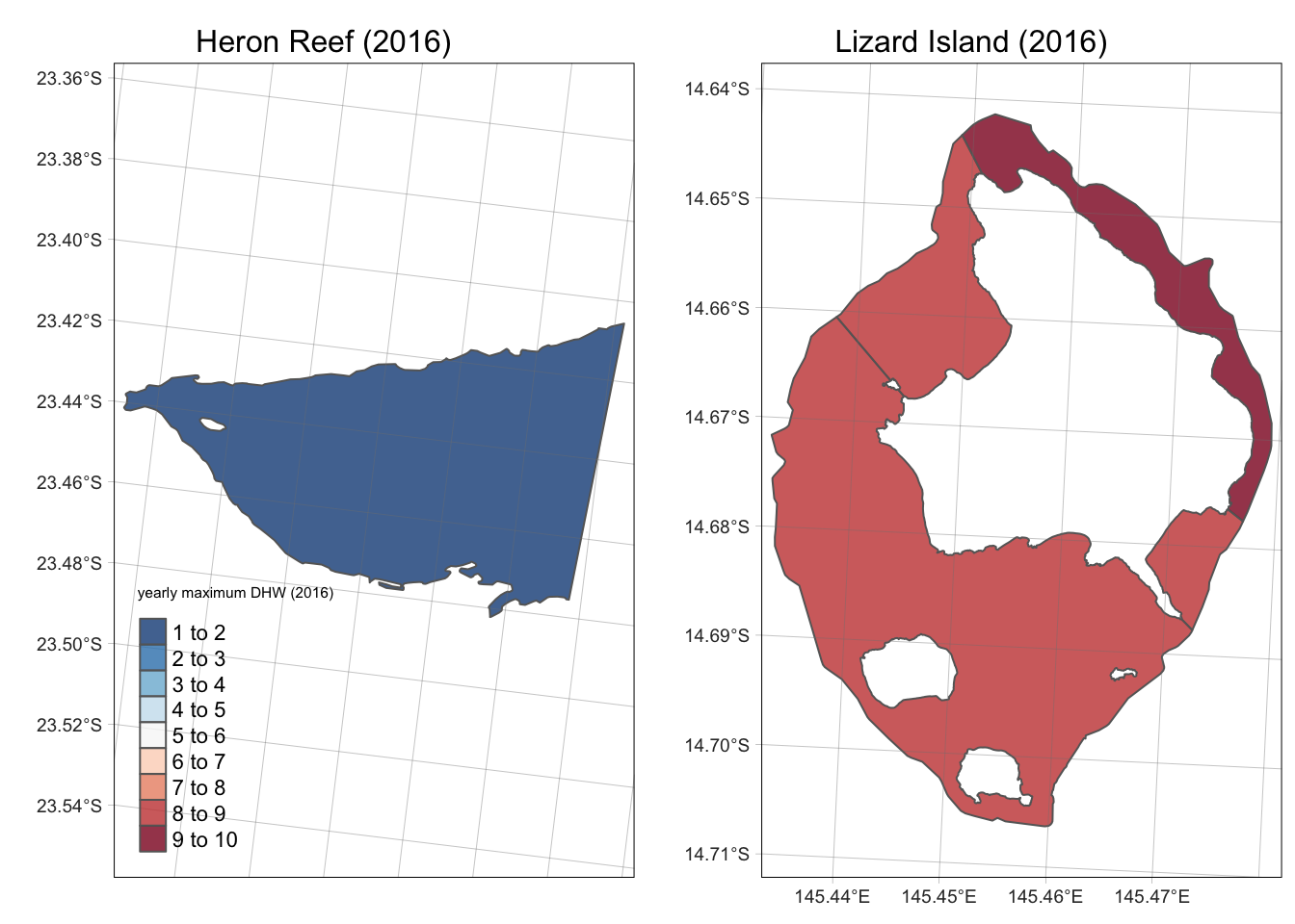
The resulting yearly maximum DHW dataset can also be filtered as a time-series to quantify the trajectories of individual reefs through time for example Heron Island in the southern GBR and Lizard Island in the northern GBR (note RdBu used over NOAA palette as it’s confusing for interspaced polygons):
dhw_subset <- gbr_shape_dhw |>
  filter(gbr_name=="Lizard Island Reef (North East)" | gbr_name=="Heron Reef") |>
  as.data.frame() |>
  dplyr::select(-id, -geometry) |>
  pivot_longer(-gbr_name, names_to="year", values_to="dhw") |>
  mutate(year = as.numeric(str_extract_all(year, "\\d+"))) |>
  arrange(gbr_name, year)

ggplot() + theme_bw() + facet_wrap(~gbr_name, ncol=2) +
  geom_smooth(data=dhw_subset, aes(x=year, y=dhw, color=gbr_name),
              method = "gam", formula = y ~ s(x, bs = "cr", k = 10), show.legend = FALSE) +
  geom_line(data=dhw_subset, aes(x=year, y=dhw, color=gbr_name), show.legend=FALSE) +
  geom_point(data=dhw_subset, aes(year, dhw, fill=gbr_name), shape=21, size=2, show.legend=FALSE) +
  theme(axis.text.x = element_text(angle = 90, vjust = 0.5, hjust=1)) +
  scale_fill_manual(values=c("aquamarine2", "coral2")) +
  scale_color_manual(values=c("aquamarine4", "coral4"))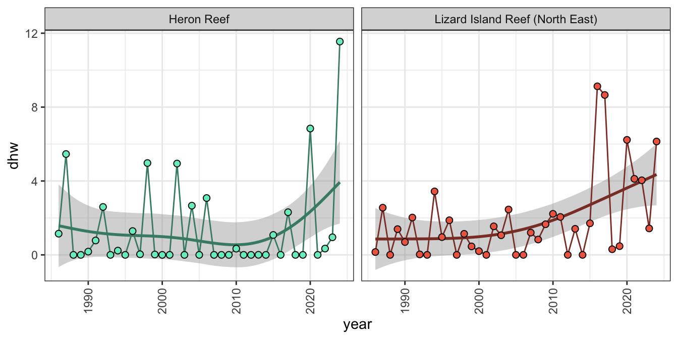
iv) validation
To check the numbers are correct, redownload the cells adjacent to Lizard Island and reprocess to get annual DHW pattern from 1986-2015 from surrounding gridcells. Max DHW closely matches the area-weighted calculations above.
  library(rerddap)
  library(lubridate)
#
#   lizard_ts_DHW <- rerddap::griddap(
#     dataset="NOAA_DHW",
#     time = c('1995-01-01','2024-04-01'),
#     latitude = c(-14.70627, -14.64135),
#     longitude = c(145.43233, 145.47928),
#     fields = c("CRW_DHW","CRW_SST","CRW_SSTANOMALY"),
#     stride = 1,
#     fmt = "csv")
#
#   lizard_ts_DHW_2 <- rerddap::griddap(
#     dataset="NOAA_DHW",
#     time = c('1986-01-01','1995-04-01'),
#     latitude = c(-14.70627, -14.64135),
#     longitude = c(145.43233, 145.47928),
#     fields = c("CRW_DHW","CRW_SST","CRW_SSTANOMALY"),
#     stride = 1,
#     fmt = "csv")
#
#   lizard_DHW <- rbind(lizard_ts_DHW_2, lizard_ts_DHW)
#   write.csv(lizard_DHW, "data/lizard_DHW.csv")


  dhw_subset_lizard <- dhw_subset |>
    filter(!gbr_name=="Heron Reef") |>
     mutate(year = as.character(year),
         time = paste0(year, "-03-01T12:00:00Z")) |>
    mutate(time=ymd_hms(time)) |>
    rename(crw_dhw=dhw)


  lizard_DHW <- read.csv("/Users/rof011/GBR-coral-bleaching/data/lizard_DHW.csv")

  lizard_DHW |>
    mutate(time=ymd_hms(time)) |>
    mutate(year= year(time)) |>
    mutate(month=month(time)) |>
    group_by(time) |>
    summarise(crw_dhw=mean(crw_dhw), crw_sst=max(crw_sst)) |>
  ggplot() + theme_bw() +
    geom_line(aes(time, crw_dhw)) +
   # geom_area(aes(time, crw_dhw), fill="darkred") +
    scale_x_datetime(date_breaks = "1 year", date_labels = "%Y") +
    theme(axis.text.x = element_text(angle = 45, hjust = 1)) +
    scale_y_continuous(limits=c(0,10), breaks=seq(0,10,2)) +
    ylab("Degree Heating Weeks")+ xlab("Year") +
    geom_point(data=dhw_subset_lizard, aes(time, crw_dhw, fill=crw_dhw), stroke=0.5, size=3, shape=21) +
    scale_fill_distiller(palette = "Reds", direction = 1, limits=c(0,10))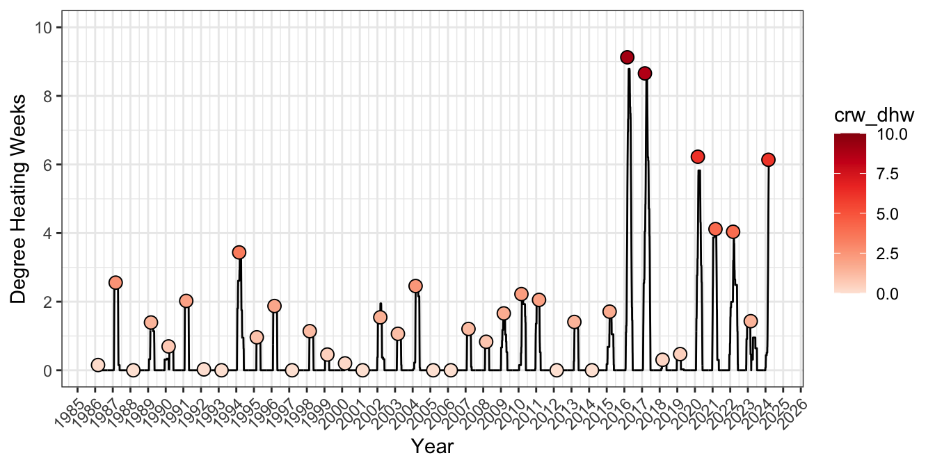
and between-cell variance explains the difference between means:
  lizard_DHW |>
    mutate(time=ymd_hms(time)) |>
    mutate(year= year(time)) |>
    mutate(month=month(time)) |>
    mutate(cell=paste0("(",longitude," / ",latitude,")")) |>
    mutate(cell=as.factor(cell)) |>
  ggplot() + theme_bw() +
    geom_line(aes(time, crw_dhw, color=cell)) +
    scale_x_datetime(date_breaks = "1 year", date_labels = "%Y") +
    theme(axis.text.x = element_text(angle = 45, hjust = 1)) +
    scale_y_continuous(limits=c(0,10), breaks=seq(0,10,2)) +
    ylab("Degree Heating Weeks")+ xlab("Year") +
    scale_color_viridis_d(direction=-1, option="C") +
    geom_point(data=dhw_subset_lizard, aes(time, crw_dhw, fill=crw_dhw), stroke=0.5, size=3, shape=21) +
    scale_fill_distiller(palette = "Reds", direction = 1, limits=c(0,10))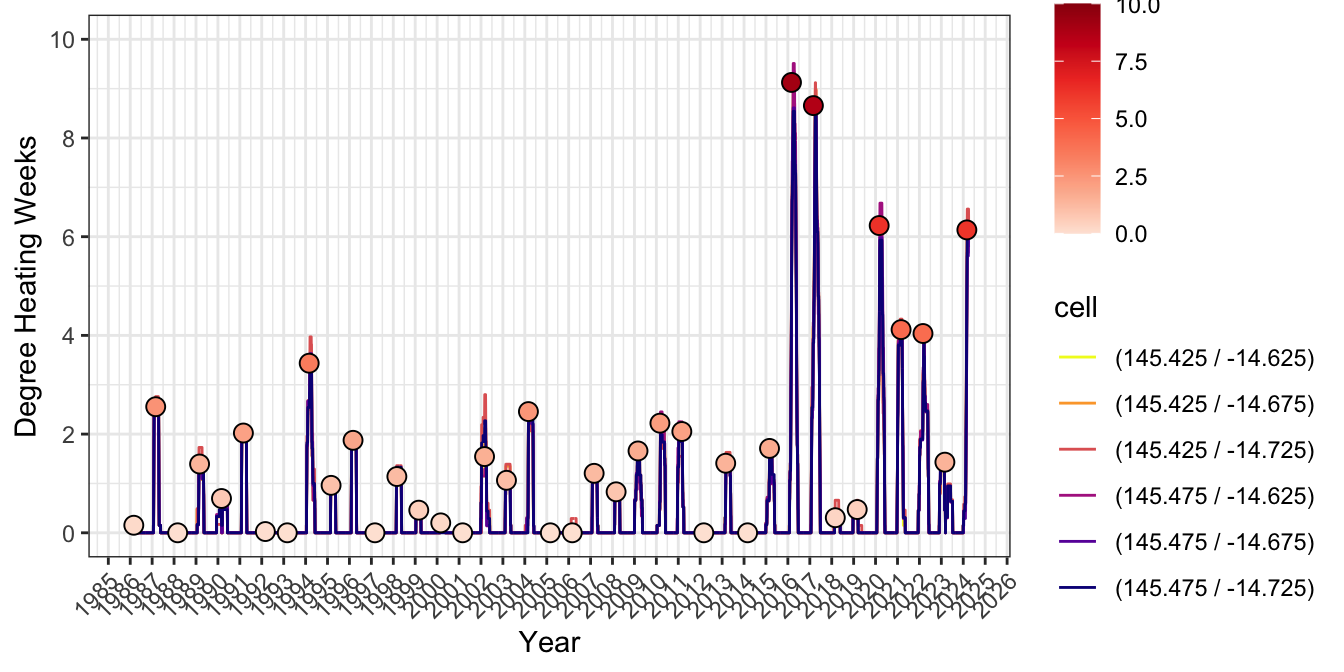
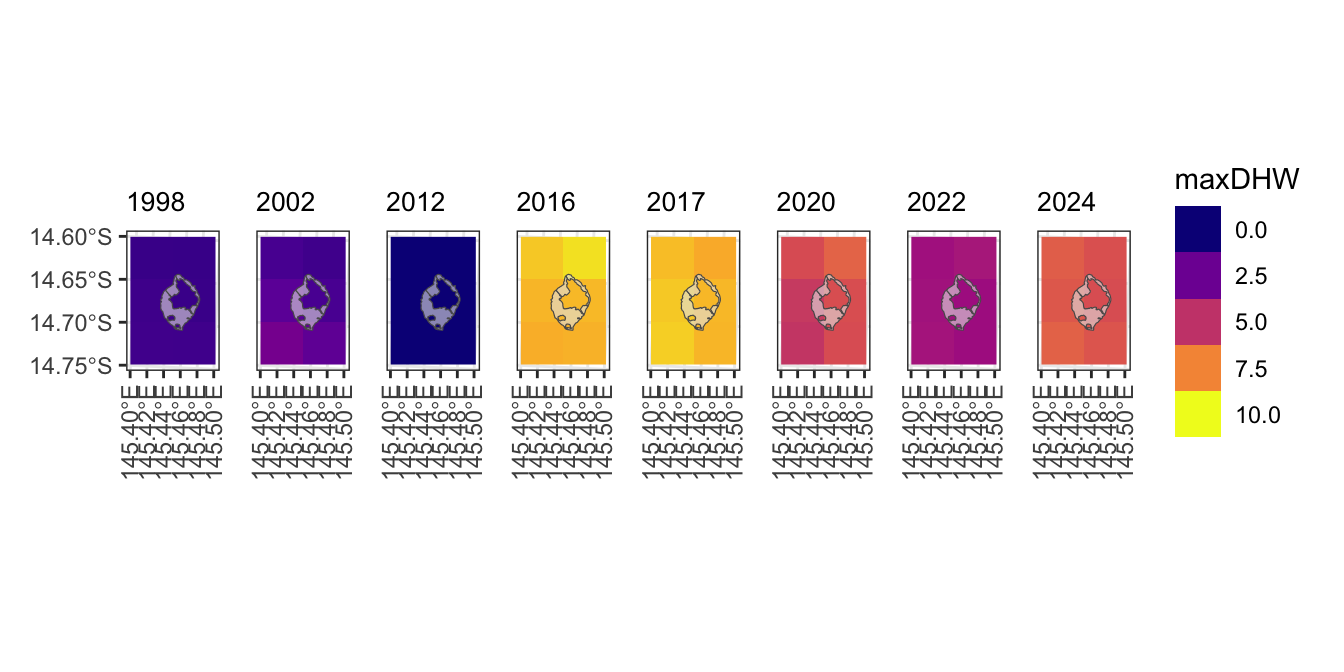
finally plot spatial maps for max DHW per year showing the area-weighted vs cell-weighted approach:
# spatial

lizard_spat <- lizard_DHW |>
    mutate(time=ymd_hms(time)) |>
    mutate(year= year(time)) |>
    group_by(year, longitude, latitude) |>
    summarise(crw_dhw=max(crw_dhw)) |>
    pivot_wider(names_from="year", values_from="crw_dhw") |>
    tidyterra::as_spatraster(crs="EPSG:4326", xycols = 1:2) |> project("EPSG:20353")

gbr_shape_dhw <- readRDS("/Users/rof011/GBR-coral-bleaching/data/gbr_shape_dhw.RDS")


lizard_shape_dhw_map <- gbr_shape_dhw %>%
  st_transform(20353) |>
  mutate(across(where(is.numeric), round, digits = 1)) |>
  filter(grepl("Lizard", gbr_name))


tmpthme <- theme(
  axis.title.y = element_blank(),
  axis.text.y = element_blank(),
  axis.ticks.y = element_blank(),
  axis.text.x = element_text(angle = 90, vjust = 0.5, hjust = 1),
  plot.title = element_text(size = 10)
)

p1998 <- ggplot() +
  theme_bw() +
  tidyterra::geom_spatraster(data = lizard_spat, aes(fill = 1998), show.legend = FALSE) +
  scale_fill_viridis_c(option = "C", limits = c(0, 10)) +
  theme(axis.text.x = element_text(angle = 90, vjust = 0.5, hjust = 1)) +
  geom_sf(data = lizard_shape_dhw_map, alpha=0.6) + ggtitle("1998") +
  theme(plot.title = element_text(size = 10))
p2002 <- ggplot() +
  theme_bw() +
  tidyterra::geom_spatraster(data = lizard_spat, aes(fill = 2002), show.legend = FALSE) +
  tmpthme +
  scale_fill_viridis_c(option = "C", limits = c(0, 10)) +
  geom_sf(data = lizard_shape_dhw_map, alpha=0.6) + ggtitle("2002")
p2012 <- ggplot() +
  theme_bw() +
  tidyterra::geom_spatraster(data = lizard_spat, aes(fill = 2012), show.legend = FALSE) +
  tmpthme +
  scale_fill_viridis_c(option = "C", limits = c(0, 10)) +
  geom_sf(data = lizard_shape_dhw_map, alpha=0.6) + ggtitle("2012")
p2016 <- ggplot() +
  theme_bw() +
  tidyterra::geom_spatraster(data = lizard_spat, aes(fill = 2016), show.legend = FALSE) +
  tmpthme +
  scale_fill_viridis_c(option = "C", limits = c(0, 10)) +
  geom_sf(data = lizard_shape_dhw_map, alpha=0.6) + ggtitle("2016")
p2017 <- ggplot() +
  theme_bw() +
  tidyterra::geom_spatraster(data = lizard_spat, aes(fill = 2017), show.legend = FALSE) +
  tmpthme +
  scale_fill_viridis_c(option = "C", limits = c(0, 10)) +
  geom_sf(data = lizard_shape_dhw_map, alpha=0.6) + ggtitle("2017")
p2020 <- ggplot() +
  theme_bw() +
  tidyterra::geom_spatraster(data = lizard_spat, aes(fill = 2020), show.legend = FALSE) +
  tmpthme +
  scale_fill_viridis_c(option = "C", limits = c(0, 10)) +
  geom_sf(data = lizard_shape_dhw_map, alpha=0.6) + ggtitle("2020")
p2022 <- ggplot() +
  theme_bw() +
  tidyterra::geom_spatraster(data = lizard_spat, aes(fill = 2022), show.legend = FALSE) +
  tmpthme +
  scale_fill_viridis_c(option = "C", limits = c(0, 10)) +
  geom_sf(data = lizard_shape_dhw_map, alpha=0.6) + ggtitle("2022")
p2024 <- ggplot() +
  theme_bw() +
  tidyterra::geom_spatraster(data = lizard_spat, aes(fill = 2024), show.legend = TRUE) +
  tmpthme +
  scale_fill_viridis_c(option = "C", limits = c(0, 10)) +
  geom_sf(data = lizard_shape_dhw_map, alpha=0.6) + ggtitle("2024") +
  guides(fill=guide_legend(title="maxDHW"))

p1998 | p2002 | p2012 | p2016 | p2017 | p2020 | p2022 | p2024