Degree Heating Weeks and mass coral bleaching on the Great Barrier Reef
George Roff
2024-03-29
Preliminary analysis of maximum Degree Heating Weeks on the Great Barrier Reef from i) the 2024 mass coral bleaching event and ii) seven mass bleaching events (1998, 2002, 2016, 2017, 2020, 2022, 2024) using the NOAA Coral Reef Watch daily satellite DHW data 1986-2024 (reef-level data based on area-weighted averages for 3,174 reefs on the GBR, see methods/code/datasets here).
1 Spatial map of Degree Heating Weeks
a) 2024 mass coral bleaching event
Map of Degree Heating Weeks (DHW) experienced during the 2024 mass coral bleaching event (01/01/24 - 01/04/24) for 3,716 reefs on the Great Barrier Reef (note DHW exceeds >12 but is limited to 0-12 DHW on the scale/legend):
library(sf)
library(ggplot2)
library(tidyverse)
library(plotly)
library(patchwork)
library(tmap)
# check NA rows - 8 NaN reef polygons, 3,716 reefs
# gbr_shape_dhw_na <- readRDS("/Users/rof011/GBR-coral-bleaching/data/gbr_shape_dhw.RDS") |>
# filter(if_any(everything(), is.na))
# load data, omit NaN as above, 3,716 reefs
gbr_shape_dhw <- readRDS("/Users/rof011/GBR-coral-bleaching/data/gbr_shape_dhw.RDS") |>
st_centroid() |>
mutate(reef_id = paste0(as.character(gbr_name), " (", id,")")) |>
filter(!if_any(everything(), is.na))
# load map files in sf from rnaturalearth:
ausmap <- rnaturalearth::ne_countries(scale="large", country="Australia") |>
st_transform(20353) |>
st_crop(gbr_shape_dhw |>
st_buffer(50000))
# map via ggplot2 and ggplotly:
# p <- ggplot() + theme_bw() +
# geom_sf(data=ausmap, fill="olivedrab4", alpha=0.2) +
# geom_sf(data=gbr_shape_dhw |>
# #mutate(dhw_max_2024=ifelse(dhw_max_2024 >12, 12, dhw_max_2024)) |>
# #select(dhw_max_2024, reef_id) |>
# mutate(max_dhw=dhw_max_2024) |>
# rename(`max DHW \n` = "dhw_max_2024"),
# aes(fill=max_dhw, text=reef_id), shape=21, stroke=0.1) +
# scale_fill_distiller(palette="RdYlBu", limits=c(0,12),
# na.value="darkred", labels=c("0","3","6","9",">12"))
dhw_colour_breaks <- c(2, 4, 8, 12, 16)
dhw_scale=c("#a5d3e5", "#eddf8c", "#ff9a15", "#820000")
p <- ggplot() + theme_bw() +
geom_sf(data=ausmap, fill="olivedrab4", alpha=0.2) +
geom_sf(data=gbr_shape_dhw |>
#mutate(dhw_max_2024=ifelse(dhw_max_2024 >16, 16, dhw_max_2024)) |>
select(dhw_max_2024, reef_id) |>
mutate(max_dhw=round(dhw_max_2024,1)) |>
rename(`max DHW \n` = "dhw_max_2024"),
aes(fill=max_dhw), shape=21, stroke=0.1) +
scale_fill_gradientn(
limits = c(0,22),
name = "max DHW",
labels = c(0, 4, 8, 12, 16),
colours = dhw_scale[c(1, seq_along(dhw_scale), length(dhw_scale))],
values = c(0, scales::rescale(dhw_colour_breaks, from = c(0,22)), 1),
)
ggplotly(p, tooltip = c("reef_id", "max_dhw")) b) 1998 - 2024 mass coral bleaching events
Comparisons of DHW experienced during the 2024 event with the previous eight mass coral bleaching events on the Great Barrier Reef (1998, 2002, 2012, 2016, 2017, 2020, 2022, 2024)
dhw_n_reefs <- gbr_shape_dhw |>
as.data.frame() |>
dplyr::select(-geometry, -id, -gbr_name) |>
pivot_longer(-c(reef_id), names_to="year", values_to="dhw_max") |>
mutate(year = as.numeric(str_extract_all(year, "\\d+"))) |>
filter(year %in% c(1998, 2002, 2016, 2017, 2020, 2022, 2024)) |>
filter(dhw_max > 4) |>
mutate(sum=n()) |>
group_by(year) %>%
summarise(count = n(), proportion=round((count/unique(sum)) *100))
#
# # 3,716 reefs
# plot1998 <- ggplot() + theme_bw() +
# theme(axis.text.x = element_text(angle = 45, hjust = 1)) +
# geom_sf(data=ausmap, fill="olivedrab4", alpha=0.2) +
# geom_sf(data=gbr_shape_dhw |>
# #mutate(dhw_max_2024=ifelse(dhw_max_2024 >12, 12, dhw_max_2024)) |>
# #select(dhw_max_2024, reef_id) |>
# mutate(max_dhw=dhw_max_1998) |>
# rename(`max DHW \n` = "dhw_max_1998"), show.legend=FALSE,
# aes(fill=max_dhw, text=reef_id), shape=21, stroke=0.1) +
# scale_fill_distiller(palette="RdYlBu", limits=c(0,12),
# na.value="darkred", labels=c("0","3","6","9",">12")) +
# ggtitle("1998")
#
#
# plot2002 <- ggplot() + theme_bw() +
# theme(axis.text.x = element_text(angle = 45, hjust = 1)) +
# geom_sf(data=ausmap, fill="olivedrab4", alpha=0.2) +
# geom_sf(data=gbr_shape_dhw |>
# #mutate(dhw_max_2024=ifelse(dhw_max_2024 >12, 12, dhw_max_2024)) |>
# #select(dhw_max_2024, reef_id) |>
# mutate(max_dhw=dhw_max_2002) |>
# rename(`max DHW \n` = "dhw_max_2002"), show.legend=FALSE,
# aes(fill=max_dhw, text=reef_id), shape=21, stroke=0.1) +
# scale_fill_distiller(palette="RdYlBu", limits=c(0,12),
# na.value="darkred", labels=c("0","3","6","9",">12")) +
# ggtitle("2002")
#
# plot2016 <- ggplot() + theme_bw() +
# theme(axis.text.x = element_text(angle = 45, hjust = 1)) +
# geom_sf(data=ausmap, fill="olivedrab4", alpha=0.2) +
# geom_sf(data=gbr_shape_dhw |>
# #mutate(dhw_max_2024=ifelse(dhw_max_2024 >12, 12, dhw_max_2024)) |>
# #select(dhw_max_2024, reef_id) |>
# mutate(max_dhw=dhw_max_2016) |>
# rename(`max DHW \n` = "dhw_max_2016"), show.legend=FALSE,
# aes(fill=max_dhw, text=reef_id), shape=21, stroke=0.1) +
# scale_fill_distiller(palette="RdYlBu", limits=c(0,12),
# na.value="darkred", labels=c("0","3","6","9",">12")) +
# ggtitle("2016")
#
#
# plot2017 <- ggplot() + theme_bw() +
# theme(axis.text.x = element_text(angle = 45, hjust = 1)) +
# geom_sf(data=ausmap, fill="olivedrab4", alpha=0.2) +
# geom_sf(data=gbr_shape_dhw |>
# #mutate(dhw_max_2024=ifelse(dhw_max_2024 >12, 12, dhw_max_2024)) |>
# #select(dhw_max_2024, reef_id) |>
# mutate(max_dhw=dhw_max_2017) |>
# rename(`max DHW \n` = "dhw_max_2017"), show.legend=FALSE,
# aes(fill=max_dhw, text=reef_id), shape=21, stroke=0.1) +
# scale_fill_distiller(palette="RdYlBu", limits=c(0,12),
# na.value="darkred", labels=c("0","3","6","9",">12")) +
# ggtitle("2017")
#
#
# plot2020 <- ggplot() + theme_bw() +
# theme(axis.text.x = element_text(angle = 45, hjust = 1)) +
# geom_sf(data=ausmap, fill="olivedrab4", alpha=0.2) +
# geom_sf(data=gbr_shape_dhw |>
# #mutate(dhw_max_2024=ifelse(dhw_max_2024 >12, 12, dhw_max_2024)) |>
# #select(dhw_max_2024, reef_id) |>
# mutate(max_dhw=dhw_max_2020) |>
# rename(`max DHW \n` = "dhw_max_2020"), show.legend=FALSE,
# aes(fill=max_dhw, text=reef_id), shape=21, stroke=0.1) +
# scale_fill_distiller(palette="RdYlBu", limits=c(0,12),
# na.value="darkred", labels=c("0","3","6","9",">12")) +
# ggtitle("2020")
#
#
# plot2022 <- ggplot() + theme_bw() +
# theme(axis.text.x = element_text(angle = 45, hjust = 1)) +
# geom_sf(data=ausmap, fill="olivedrab4", alpha=0.2) +
# geom_sf(data=gbr_shape_dhw |>
# #mutate(dhw_max_2024=ifelse(dhw_max_2024 >12, 12, dhw_max_2024)) |>
# #select(dhw_max_2024, reef_id) |>
# mutate(max_dhw=dhw_max_2022) |>
# rename(`max DHW \n` = "dhw_max_2022"), show.legend=FALSE,
# aes(fill=max_dhw, text=reef_id), shape=21, stroke=0.1) +
# scale_fill_distiller(palette="RdYlBu", limits=c(0,12),
# na.value="darkred", labels=c("0","3","6","9",">12")) +
# ggtitle("2022")
#
# plot2024 <- ggplot() + theme_bw() +
# theme(axis.text.x = element_text(angle = 45, hjust = 1)) +
# geom_sf(data=ausmap, fill="olivedrab4", alpha=0.2) +
# geom_sf(data=gbr_shape_dhw |>
# #mutate(dhw_max_2024=ifelse(dhw_max_2024 >12, 12, dhw_max_2024)) |>
# #select(dhw_max_2024, reef_id) |>
# mutate(max_dhw=dhw_max_2024) |>
# rename(`max DHW \n` = "dhw_max_2024"), show.legend=FALSE,
# aes(fill=max_dhw, text=reef_id), shape=21, stroke=0.1) +
# scale_fill_distiller(palette="RdYlBu", limits=c(0,12),
# na.value="darkred", labels=c("0","3","6","9",">12")) +
# ggtitle("2024")
#
# plot20XX <- ggplot() + theme_bw() +
# theme(axis.text.x = element_text(angle = 45, hjust = 1)) +
# geom_sf(data=ausmap, fill="olivedrab4", linewidth=0,alpha=0) +
# theme(panel.grid.major = element_blank(),
# panel.grid.minor = element_blank(),
# axis.title.x = element_blank(),
# axis.title.y = element_blank(),
# axis.text.x = element_blank(),
# axis.text.y = element_blank())
# (plot1998|plot2002)/
# (plot2016|plot2017|plot2020)/
# (plot2022|plot2024|plot20XX)
# 3,716 reefs
plot1998 <-
gbr_shape_dhw |>
mutate(max_dhw=dhw_max_1998) |>
mutate(dhw_bins=cut(max_dhw, breaks=c(-0.01,4,8,12,16,20),
labels=c("0-4 DHW", "4-8 DHW", "8-12 DHW", "12-16 DHW", "16-20 DHW"))) |>
rename(`max DHW \n` = "dhw_max_2024") |>
ggplot() + theme_bw() + #facet_wrap(~dhw_bins) +
theme(axis.text.x = element_text(angle = 45, hjust = 1)) +
geom_sf(aes(fill=max_dhw), alpha=0, show.legend=FALSE) +
geom_sf(data=ausmap, fill="olivedrab4", alpha=0.2) +
geom_sf(aes(fill=max_dhw), shape=21, stroke=0.1, show.legend=FALSE) +
scale_fill_gradientn(
limits = c(0,22),
name = "max DHW",
labels = c(0, 4, 8, 12, 16),
colours = dhw_scale[c(1, seq_along(dhw_scale), length(dhw_scale))],
values = c(0, scales::rescale(dhw_colour_breaks, from = c(0,22)), 1),
) + ggtitle("1998")
plot2002 <-
gbr_shape_dhw |>
mutate(max_dhw=dhw_max_2002) |>
mutate(dhw_bins=cut(max_dhw, breaks=c(-0.01,4,8,12,16,20),
labels=c("0-4 DHW", "4-8 DHW", "8-12 DHW", "12-16 DHW", "16-20 DHW"))) |>
rename(`max DHW \n` = "dhw_max_2024") |>
ggplot() + theme_bw() + #facet_wrap(~dhw_bins) +
theme(axis.text.x = element_text(angle = 45, hjust = 1)) +
geom_sf(aes(fill=max_dhw), alpha=0, show.legend=FALSE) +
geom_sf(data=ausmap, fill="olivedrab4", alpha=0.2) +
geom_sf(aes(fill=max_dhw), shape=21, stroke=0.1, show.legend=FALSE) +
scale_fill_gradientn(
limits = c(0,22),
name = "max DHW",
labels = c(0, 4, 8, 12, 16),
colours = dhw_scale[c(1, seq_along(dhw_scale), length(dhw_scale))],
values = c(0, scales::rescale(dhw_colour_breaks, from = c(0,22)), 1),
) + ggtitle("2002")
plot2016 <-
gbr_shape_dhw |>
mutate(max_dhw=dhw_max_2016) |>
mutate(dhw_bins=cut(max_dhw, breaks=c(-0.01,4,8,12,16,20),
labels=c("0-4 DHW", "4-8 DHW", "8-12 DHW", "12-16 DHW", "16-20 DHW"))) |>
rename(`max DHW \n` = "dhw_max_2024") |>
ggplot() + theme_bw() + #facet_wrap(~dhw_bins) +
theme(axis.text.x = element_text(angle = 45, hjust = 1)) +
geom_sf(aes(fill=max_dhw), alpha=0, show.legend=FALSE) +
geom_sf(data=ausmap, fill="olivedrab4", alpha=0.2) +
geom_sf(aes(fill=max_dhw), shape=21, stroke=0.1, show.legend=FALSE) +
scale_fill_gradientn(
limits = c(0,22),
name = "max DHW",
labels = c(0, 4, 8, 12, 16),
colours = dhw_scale[c(1, seq_along(dhw_scale), length(dhw_scale))],
values = c(0, scales::rescale(dhw_colour_breaks, from = c(0,22)), 1),
) + ggtitle("2016")
plot2017 <-
gbr_shape_dhw |>
mutate(max_dhw=dhw_max_2017) |>
mutate(dhw_bins=cut(max_dhw, breaks=c(-0.01,4,8,12,16,20),
labels=c("0-4 DHW", "4-8 DHW", "8-12 DHW", "12-16 DHW", "16-20 DHW"))) |>
rename(`max DHW \n` = "dhw_max_2024") |>
ggplot() + theme_bw() + #facet_wrap(~dhw_bins) +
theme(axis.text.x = element_text(angle = 45, hjust = 1)) +
geom_sf(aes(fill=max_dhw), alpha=0, show.legend=FALSE) +
geom_sf(data=ausmap, fill="olivedrab4", alpha=0.2) +
geom_sf(aes(fill=max_dhw), shape=21, stroke=0.1, show.legend=FALSE) +
scale_fill_gradientn(
limits = c(0,22),
name = "max DHW",
labels = c(0, 4, 8, 12, 16),
colours = dhw_scale[c(1, seq_along(dhw_scale), length(dhw_scale))],
values = c(0, scales::rescale(dhw_colour_breaks, from = c(0,22)), 1),
) + ggtitle("2017")
plot2020 <-
gbr_shape_dhw |>
mutate(max_dhw=dhw_max_2020) |>
mutate(dhw_bins=cut(max_dhw, breaks=c(-0.01,4,8,12,16,20),
labels=c("0-4 DHW", "4-8 DHW", "8-12 DHW", "12-16 DHW", "16-20 DHW"))) |>
rename(`max DHW \n` = "dhw_max_2024") |>
ggplot() + theme_bw() + #facet_wrap(~dhw_bins) +
theme(axis.text.x = element_text(angle = 45, hjust = 1)) +
geom_sf(aes(fill=max_dhw), alpha=0, show.legend=FALSE) +
geom_sf(data=ausmap, fill="olivedrab4", alpha=0.2) +
geom_sf(aes(fill=max_dhw), shape=21, stroke=0.1, show.legend=FALSE) +
scale_fill_gradientn(
limits = c(0,22),
name = "max DHW",
labels = c(0, 4, 8, 12, 16),
colours = dhw_scale[c(1, seq_along(dhw_scale), length(dhw_scale))],
values = c(0, scales::rescale(dhw_colour_breaks, from = c(0,22)), 1),
) + ggtitle("2020")
plot2022 <-
gbr_shape_dhw |>
mutate(max_dhw=dhw_max_2022) |>
mutate(dhw_bins=cut(max_dhw, breaks=c(-0.01,4,8,12,16,20),
labels=c("0-4 DHW", "4-8 DHW", "8-12 DHW", "12-16 DHW", "16-20 DHW"))) |>
rename(`max DHW \n` = "dhw_max_2024") |>
ggplot() + theme_bw() + #facet_wrap(~dhw_bins) +
theme(axis.text.x = element_text(angle = 45, hjust = 1)) +
geom_sf(aes(fill=max_dhw), alpha=0, show.legend=FALSE) +
geom_sf(data=ausmap, fill="olivedrab4", alpha=0.2) +
geom_sf(aes(fill=max_dhw), shape=21, stroke=0.1, show.legend=FALSE) +
scale_fill_gradientn(
limits = c(0,22),
name = "max DHW",
labels = c(0, 4, 8, 12, 16),
colours = dhw_scale[c(1, seq_along(dhw_scale), length(dhw_scale))],
values = c(0, scales::rescale(dhw_colour_breaks, from = c(0,22)), 1),
) + ggtitle("2022")
plot2024 <-
gbr_shape_dhw |>
mutate(max_dhw=dhw_max_2024) |>
mutate(dhw_bins=cut(max_dhw, breaks=c(-0.01,4,8,12,16,20),
labels=c("0-4 DHW", "4-8 DHW", "8-12 DHW", "12-16 DHW", "16-20 DHW"))) |>
rename(`max DHW \n` = "dhw_max_2024") |>
ggplot() + theme_bw() + #facet_wrap(~dhw_bins) +
theme(axis.text.x = element_text(angle = 45, hjust = 1)) +
geom_sf(aes(fill=max_dhw), alpha=0, show.legend=FALSE) +
geom_sf(data=ausmap, fill="olivedrab4", alpha=0.2) +
geom_sf(aes(fill=max_dhw), shape=21, stroke=0.1, show.legend=FALSE) +
scale_fill_gradientn(
limits = c(0,22),
name = "max DHW",
labels = c(0, 4, 8, 12, 16),
colours = dhw_scale[c(1, seq_along(dhw_scale), length(dhw_scale))],
values = c(0, scales::rescale(dhw_colour_breaks, from = c(0,22)), 1),
) + ggtitle("2024")
plot20XX <- ggplot() + theme_bw() +
theme(axis.text.x = element_text(angle = 45, hjust = 1)) +
geom_sf(data=ausmap, fill="olivedrab4", linewidth=0,alpha=0) +
theme(panel.grid.major = element_blank(),
panel.grid.minor = element_blank(),
axis.title.x = element_blank(),
axis.title.y = element_blank(),
axis.text.x = element_blank(),
axis.text.y = element_blank())
(plot1998|plot2002|plot2016|plot2017)/
(plot2020|plot2022|plot2024|plot20XX)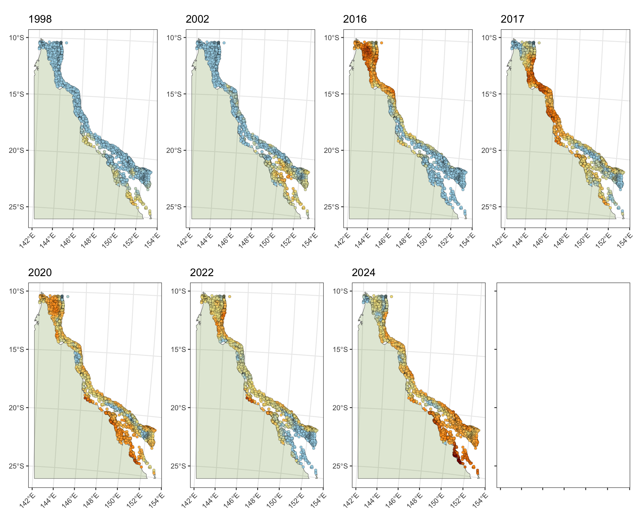
2) Increasing frequency and intensity of max Degree Heating Weeks
Using yearly maximum DHW to compare changes in the distributions of DHW across 3,716 reefs on the GBR:
a) DHW distributions
Changes in distributions of Degree Heating Weeks per reef over time during the seven mass coral bleaching events (1998, 2002, 2016, 2017, 2020, 2022, 2024)
library(sf)
library(ggplot2)
library(tidyverse)
# extract median DHW and max DHW for each bleaching event
dhw_subset_bleaching_dhw <- gbr_shape_dhw |>
as.data.frame() |>
dplyr::select(-geometry, -id, -gbr_name) |>
pivot_longer(-c(reef_id), names_to="year", values_to="dhw_max") |>
mutate(year = as.numeric(str_extract_all(year, "\\d+"))) |>
# mutate(reef_id = paste0(as.character(gbr_name), " (", id,")")) |>
arrange(reef_id, year) |>
filter(year %in% c(1998,2002,2016,2017,2020,2022,2024)) |>
group_by(year) |>
mutate(mean_dhw_max = round(median(dhw_max, na.rm=TRUE),1)) |>
mutate(mean_dhw_max_text= paste0("Median = ", round(mean_dhw_max, 1), " DHW"))
# 3,716 reefs (reef_id) - 26,012 rows
# unique(dhw_subset_bleaching_dhw$reef_id) |> length()
ggplot() + theme_bw() +
ggridges::stat_density_ridges(data=dhw_subset_bleaching_dhw, alpha=0.8, scale=1.2, size=0.3,
aes(y=as.factor(year), x=dhw_max, fill=mean_dhw_max),
rel_min_height=0.00001,
quantiles = c(0.05, 0.25, 0.5, 0.75, 0.95),
quantile_lines = TRUE, #quantile_fun = mean,
vline_color = c("black"), vline_width = 2, show.legend=FALSE) +
scale_fill_distiller(palette = "Reds", direction = 1, name="median\nmax_DHW\nper reef") +
scale_color_distiller(palette = "Reds", direction = 1, name="median\nmax_DHW\nper reef", limits=c(0,8)) +
geom_text(data=dhw_subset_bleaching_dhw, nudge_y=0.15, nudge_x=1.75, size=3,
aes(x=16, y=as.factor(year), color=mean_dhw_max, label=mean_dhw_max_text)) +
xlab("Maximum DHW per reef") + ylab("Mass bleaching event") +
theme(panel.grid.major.x = element_blank(), panel.grid.minor.x = element_blank())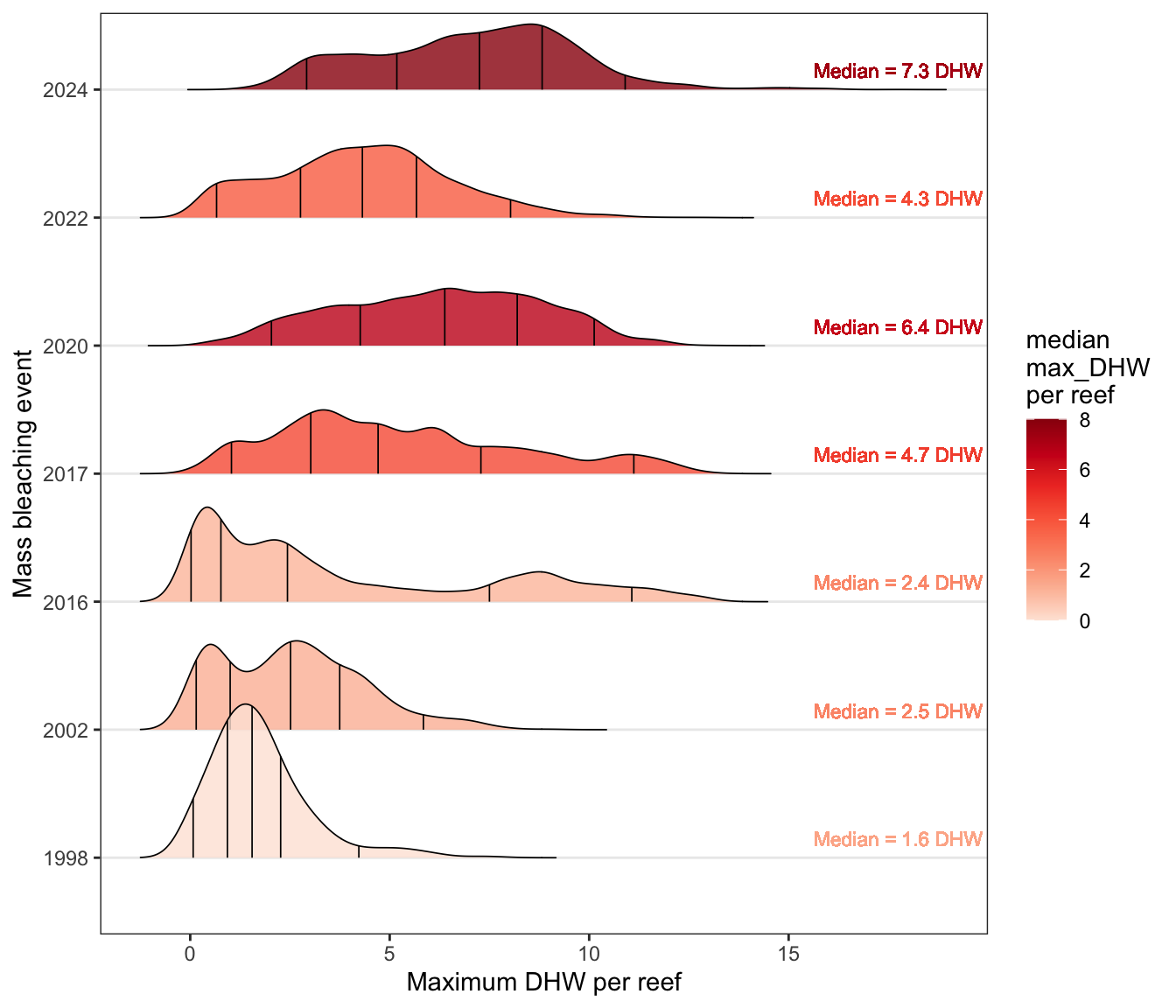
b) DHW frequencies
Changes in distributions of Degree Heating Weeks per reef during the seven mass coral bleaching events (1998, 2002, 2016, 2017, 2020, 2022, 2024):
b <- ggplot() + theme_bw() +
ggbeeswarm::geom_quasirandom(data=dhw_subset_bleaching_dhw |> mutate(dhw_max=round(dhw_max,1)), alpha=0.8, scale=1.2, size=0.3, method="tukeyDense",
aes(y=as.factor(year), x=dhw_max, color=dhw_max, text=reef_id) , rel_min_height=0.00001,
quantiles = c(0.5), quantile_lines = FALSE, quantile_fun = median,
vline_color = c("white"), vline_width = 2, show.legend=FALSE) +
scale_color_distiller(palette = "Reds", direction = 1, name="mean\nmax_DHW\nper reef") +
xlab("Maximum DHW per reef") + ylab("Mass bleaching event") +
theme(panel.grid.major.x = element_blank(), panel.grid.minor.x = element_blank())
b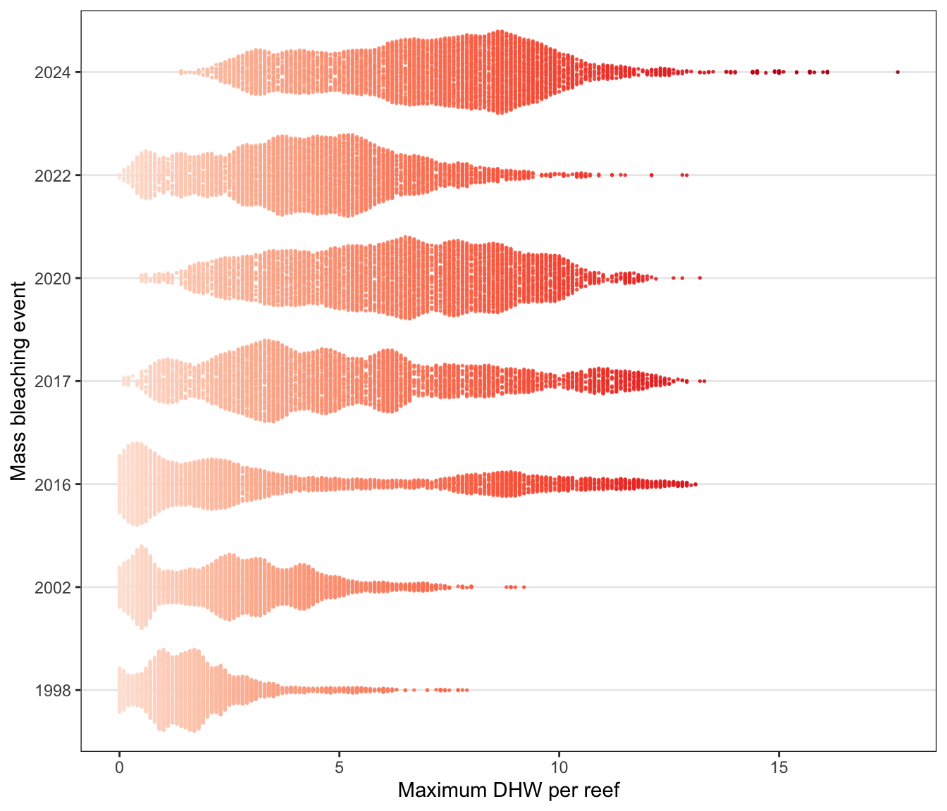
#ggplotly(b, tooltip = c("reef_id", "dhw_max")) 3. Shifts in thermal stress during mass coral bleaching events (1998-2024)
Timing (year) of the highest maximum DHW per reef (3,174 reefs) and comparisons of DHW category frequency (<1 DHW, 1-4 DHW, 4-8 DHW, 8-12 DHW, 12-16 DHW, 16-20 DHW) between the seven mass coral bleaching events on the GBR:
a) Highest Maximum Degree Heating Weeks
Year in which the highest maximum DHW was experienced for each of the 3,716 reefs:
- 46% of reefs on the GBR experienced record max DHW in the 2024 event, with the majority of these reefs in the southern GBR region.
dhw_subset_bleaching_topn <- gbr_shape_dhw |>
as.data.frame() |>
dplyr::select(-geometry, -id, -gbr_name) |>
pivot_longer(-c(reef_id), names_to="year", values_to="dhw_max") |>
group_by(reef_id) |>
top_n(n=1)
# unique(dhw_subset_bleaching_topn$year)
# [1] "dhw_max_1987" "dhw_max_2020" "dhw_max_2024" "dhw_max_2017"
# "dhw_max_2016" "dhw_max_2002" "dhw_max_2022" "dhw_max_2021"
dhw_subset_bleaching_topn <- dhw_subset_bleaching_topn |>
mutate(year = as.factor(str_extract_all(year, "\\d+"))) |>
mutate(year=factor(year, c("1987", "2002", "2012", "2016", "2017", "2020", "2021", "2022", "2024"))) |>
filter(year %in% c("1987", "2002", "2016", "2017", "2020", "2021", "2022", "2024"))
year_counts <- dhw_subset_bleaching_topn %>%
group_by(year) %>%
summarise(count = n(), proportion=round((count/nrow(dhw_subset_bleaching_topn)) *100)) |>
mutate(proportionlabel=paste0("(", count, ")"))
# Step 2 & 3: Create the histogram and add text annotations for proportions
hist <- ggplot() + theme_bw() +
geom_col(data=year_counts, aes(x=as.factor(year), fill=as.factor(year), y=proportion),
color="black", linewidth=0.2, show.legend=FALSE) +
geom_text(data=year_counts, aes(x=year, y=proportion, label=proportionlabel),
size=3, vjust=-0.5, color="black") + ylab("Proportion of reefs (%)") + xlab("\nYear") +
scale_fill_manual(values=c("#8898d8","#8898d8", "#89d3db", "#74b9e6", "#cdd888", "#aed588", "#aed588", "#ea7575")) + ylim(0,50) +
theme(panel.grid.major.x = element_blank(),
panel.grid.major.y = element_line( size=0.025, color="black"))
dhw_subset_bleaching_topn_map <- left_join(gbr_shape_dhw |> select(reef_id), dhw_subset_bleaching_topn, by="reef_id")
map <- ggplot() + theme_bw() +
geom_sf(data=ausmap, fill="olivedrab4", alpha=0.2) +
geom_sf(data=dhw_subset_bleaching_topn_map, aes(fill=year), shape=21, stroke=0.1, show.legend=FALSE) +
scale_fill_manual(values=c("#8898d8","#8898d8", "#89d3db", "#74b9e6", "#cdd888", "#aed588", "#aed588", "#ea7575"))
hist | map 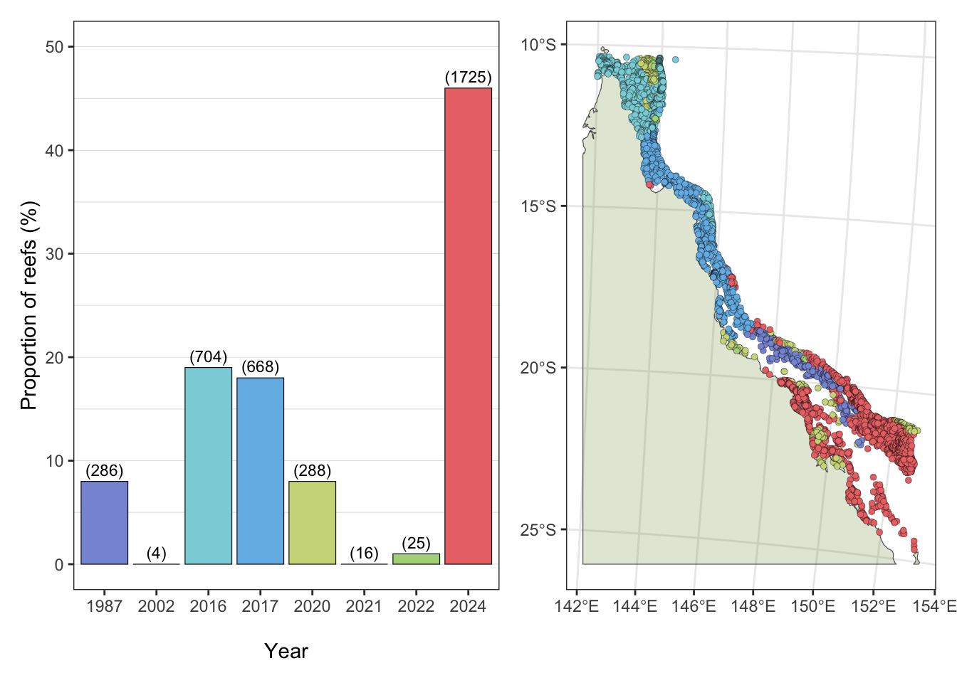
b) Increasing frequency of DHW through time
- Total number of reefs exposed to >4DHW in each of the seven previous mass bleaching events (R2 = 0.83):
gbr_shape_dhw |>
as.data.frame() |>
dplyr::select(-geometry, -id, -gbr_name) |>
pivot_longer(-c(reef_id), names_to="year", values_to="dhw_max") |>
mutate(year = as.numeric(str_extract_all(year, "\\d+"))) |>
filter(year %in% c(1998, 2002, 2016, 2017, 2020, 2022, 2024)) |>
filter(dhw_max > 4) |>
group_by(year) %>%
summarise(count = n(),
proportion=((count/length(unique(gbr_shape_dhw$reef_id)))*100)) |>
mutate(count=paste0(paste0("(n=", count,")"))) |>
ggplot() + theme_bw() +
geom_point(aes(year, proportion, fill=proportion), shape=21, size=3.5,
show.legend=FALSE) +
geom_smooth(aes(year, proportion),
method="lm", se = FALSE,
#method = "gam", formula = y ~ s(x, bs = "cr", k = 3), se = FALSE,
show.legend = FALSE, linewidth=0.09) +
theme(axis.text.x = element_text(angle = 90, vjust = 0.5, hjust=1)) +
geom_text(aes(year, proportion, label=count), nudge_y=-5, nudge_x=0, size=2.5) +
geom_text(aes(year, proportion, label=c("1998", "2012", "2016", "2017",
"2020", "2022", "2024")), nudge_y=5, nudge_x=0, size=3) +
scale_x_continuous(breaks=seq(1996, 2026,4), limits=c(1996, 2026)) +
scale_y_continuous(breaks=seq(0, 100, 20), limits=c(0, 100)) +
xlab("\nMass bleaching event Year") + ylab("Proportion of reefs impacted by >4DHW") +
scale_fill_distiller(palette = "Reds", direction = 1, limits=c(0,100)) 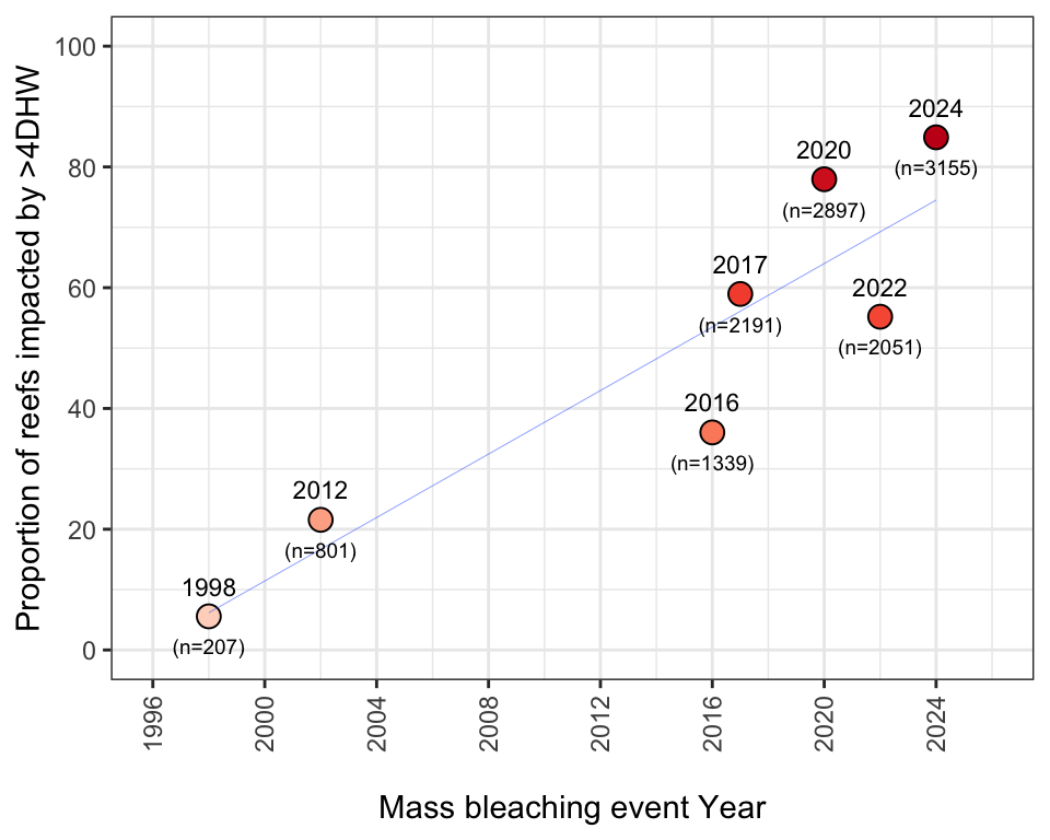
# max_dhw_data <- gbr_shape_dhw |>
# as.data.frame() |>
# dplyr::select(-geometry, -id, -gbr_name) |>
# pivot_longer(-c(reef_id), names_to="year", values_to="dhw_max") |>
# mutate(year = as.numeric(str_extract_all(year, "\\d+"))) |>
# filter(year %in% c(1998, 2002, 2016, 2017, 2020, 2022, 2024)) |>
# filter(dhw_max > 4) |>
# group_by(year) %>%
# summarise(count = n(),
# proportion=((count/length(unique(gbr_shape_dhw$reef_id)))*100)) #|>
# # mutate(count=paste0(paste0("(n=", count,")")))
# summary(lm(count~year, data=max_dhw_data))c) Increasing intensity of DHW through time
- Shifts in DHW categories across the seven mass coral bleaching events indicates increasing intensity of DHW since the first event in 1998:
dhw_subset_bleaching_dhw |> # 25,598 reefs with na_omit()
mutate(bins = cut(dhw_max, seq(0,20,4))) |>
mutate(namebins = cut(dhw_max, seq(0,20,4),
labels=c("<1 DHW", "4-8 DHW", "8-12 DHW",
"12-16 DHW", "16-20 DHW"))) |>
mutate(namebins = cut(dhw_max, c(0, 1, 4, 8, 12, 16, 20),
labels=c("<1 DHW", "1-4 DHW", "4-8 DHW",
"8-12 DHW", "12-16 DHW", "16-20 DHW"))) |>
na.omit() |>
ggplot() + theme_bw() + facet_wrap(~year, nrow=1) +
geom_histogram(aes(x=as.factor(namebins), y=(after_stat(count / sum(count))*700), fill=namebins),
stat="count", color="black", show.legend=FALSE) + ylim(0,100) +
geom_text(stat='count', aes(x=namebins, y=((..count.. / sum(..count..)) * 700),
label=ifelse((..count../sum(..count..)) < 0.01,
sprintf("%.1f%%", 100 * ..count../sum(..count..)), "")),
nudge_x=0.4, nudge_y=11, vjust=-0.5, angle=90, color="grey20", size=3.5) +
theme(axis.text.x = element_text(angle = 60, hjust = 1)) +
geom_text(stat='count', aes(x=namebins, y=((..count.. / sum(..count..)) * 700),
label=ifelse((..count../sum(..count..)) > 0.01,
sprintf("%.0f%%", 100 * ..count../sum(..count..)), "")),
nudge_x=0.4, nudge_y=8, vjust=-0.5, angle=90, color="grey20", size=3.5) +
theme(axis.text.x = element_text(angle = 60, hjust = 1)) +
ylab("Proportion of reefs") + xlab("\n Degree Heating Weeks") +
#scale_fill_manual(values=c("#d6e8f1", "#f9f2b7", "#f5c082","#d56245", "#a32208", "#820000"))
scale_fill_manual(values=c("#a5d3e5", "#eddf8c", "#efa760","#d56245", "#a32208", "#820000"))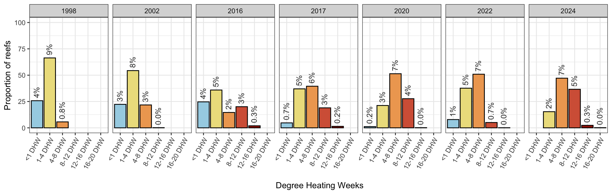
No thermal stress (<1DHW) and mild thermal stress (<4 DHW) have decreased since 1998, with increases in the moderate (4-8DHW) increasingly severe categories (8-12DHW, 12-16DHW) and the “new” category “severe” bleaching in 2024 (16-20DHW) :
dhw_subset_bleaching_dhw |>
mutate(bins = cut(dhw_max, seq(0,20,4))) |>
mutate(namebins = cut(dhw_max, seq(0,20,4),
labels=c("Unimpacted (<1 DHW)", "4-8 DHW",
"8-12 DHW", "12-16 DHW", "16-20 DHW"))) |>
mutate(namebins = cut(dhw_max, c(0, 1, 4, 8, 12, 16, 20),
labels=c("<1 DHW", "1-4 DHW", "4-8 DHW",
"8-12 DHW", "12-16 DHW", "16-20 DHW"))) |>
na.omit() |>
ggplot() + theme_bw() + facet_wrap(~namebins, nrow=1) +
geom_histogram(aes(x=as.factor(year), y=(after_stat(count / sum(count))*700), fill=namebins),
stat="count", color="black", show.legend=FALSE) + ylim(0,100) +
geom_text(stat='count', aes(x=as.factor(year), y=((..count.. / sum(..count..)) * 700),
label=ifelse((..count../sum(..count..)) < 0.01,
sprintf("%.1f%%", 100 * ..count../sum(..count..)), "")),
nudge_x=0.4, nudge_y=11, vjust=-0.5, angle=90, color="grey20", size=3.5) +
theme(axis.text.x = element_text(angle = 60, hjust = 1)) +
geom_text(stat='count', aes(x=as.factor(year), y=((..count.. / sum(..count..)) * 700),
label=ifelse((..count../sum(..count..)) > 0.01,
sprintf("%.0f%%", 100 * ..count../sum(..count..)), "")),
nudge_x=0.4, nudge_y=8, vjust=-0.5, angle=90, color="grey20", size=3.5) +
theme(axis.text.x = element_text(angle = 60, hjust = 1)) +
ylab("Proportion of reefs") + xlab("\n Degree Heating Weeks") +
# scale_fill_manual(values=c("#d6e8f1", "#f9f2b7", "#f5c082","#d56245", "#a32208", "#820000"))
scale_fill_manual(values=c("#a5d3e5", "#eddf8c", "#efa760","#d56245", "#a32208", "#820000"))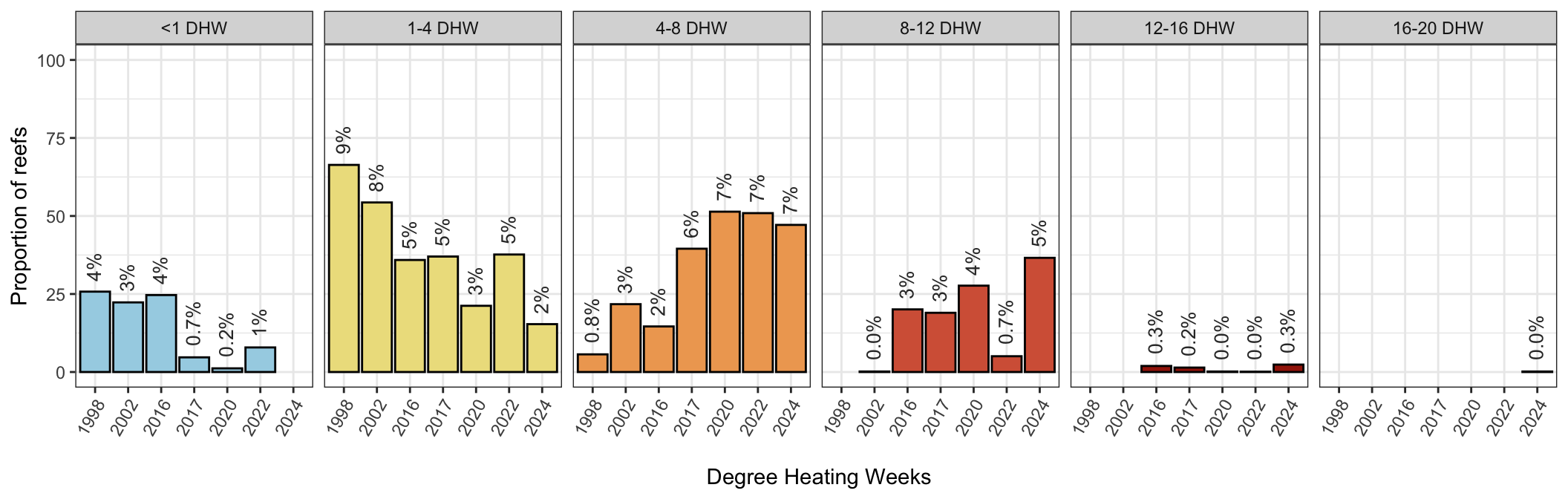
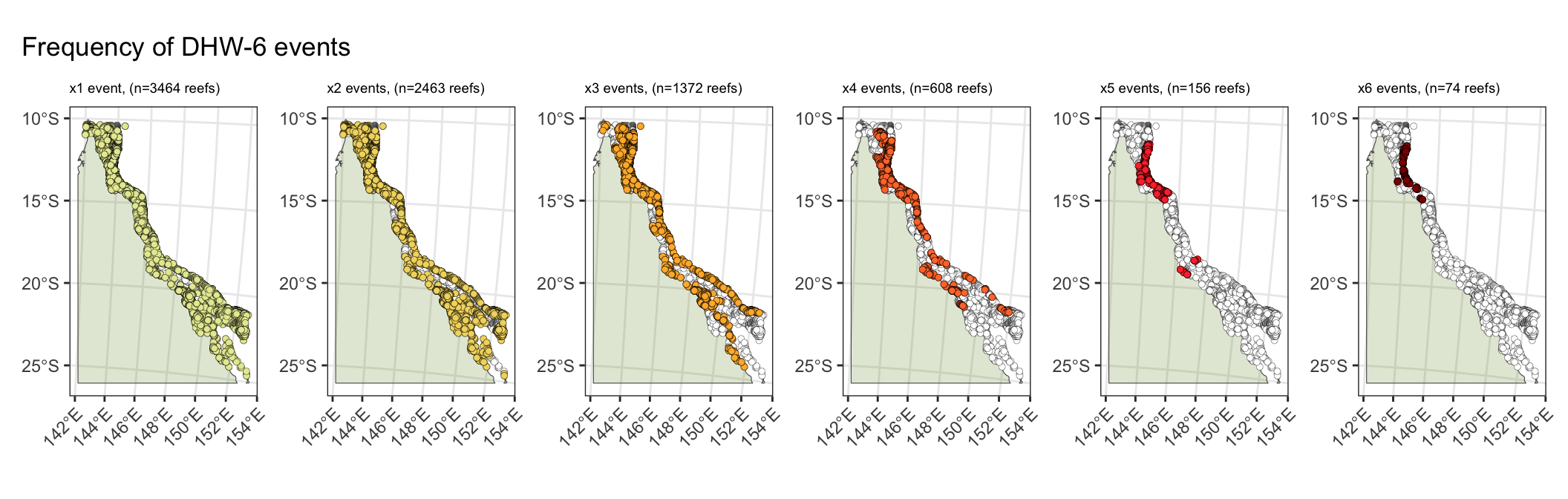
4) Recurrent thermal stress over the past decade
The Great Barrier Reef has experienced five mass bleaching events (2016, 2017, 2020, 2022, 2024) in the past decade.
- A total of 93% of reefs have experienced at least one thermal stress event of >6 DHW.
- A third of reefs (37%) have been exposed to three >6DHW events in the last decade, with these events impacting reefs across the length of the GBR (North-South).
- A subset of reefs (608 reefs, 16% of all reefs) have been exposed to recurrent thermal stress events of four >6DHW events (16%).
- Severe repeat thermal stress has to date been limited to the northern GBR, with 5% of reefs (n=156) exposed to five >6DHW events and ~2.5% of reefs (n=74) exposed to six >6DHW events.
### DHW 6 once
dhw_impacted_reefs <- gbr_shape_dhw |>
na.omit() |>
as.data.frame() |>
dplyr::select(-geometry, -id, -gbr_name) |>
pivot_longer(-c(reef_id), names_to="year", values_to="dhw_max") |>
mutate(year = as.numeric(substr(year, nchar(year)-3, nchar(year)))) |>
filter(dhw_max>6) |>
filter(year>2014) |>
group_by(reef_id) |>
mutate(count=n())
# 1 event
dhw_events_1 <- dhw_impacted_reefs |> filter(count>=1) %>%
left_join(gbr_shape_dhw |> select(reef_id),., by="reef_id") |>
mutate(impact = ifelse(is.na(count), "unimpacted", "impacted")) |>
arrange(desc(impact))
dhw_events_1_nreefs <-dhw_impacted_reefs |>
na.omit() |>
filter(count >= 1) |>
distinct(reef_id) |>
summarise(unique_reef_count = n()) |>
nrow()
dhw_6_1 <- ggplot() + theme_bw() +
geom_sf(data=ausmap, fill="olivedrab4", alpha=0.2) +
geom_sf(data=dhw_events_1, aes(fill=impact), shape=21, stroke=0.1, show.legend=FALSE) +
scale_fill_manual(values=c("#e6eaa0", "white")) +
theme(axis.text.x = element_text(angle = 45, hjust = 1)) +
ggtitle(paste0("x1 event, (n=", dhw_events_1_nreefs, " reefs)")) +
theme(plot.title = element_text(size = 7))
# 2 events
dhw_events_2 <- dhw_impacted_reefs |>
mutate(reef_id=as.factor(reef_id)) |>
filter(count>=2) %>%
left_join(gbr_shape_dhw |> select(reef_id),., by="reef_id") |>
mutate(impact = ifelse(is.na(count), "unimpacted", "impacted")) |>
arrange(desc(impact))
dhw_events_2_nreefs <-dhw_impacted_reefs |>
filter(count >= 2) |>
distinct(reef_id) |>
summarise(unique_reef_count = n()) |>
nrow()
dhw_6_2 <- ggplot() + theme_bw() +
geom_sf(data=ausmap, fill="olivedrab4", alpha=0.2) +
geom_sf(data=dhw_events_2, aes(fill=impact), shape=21, stroke=0.1, show.legend=FALSE) +
scale_fill_manual(values=c("#f2d86d", "white")) +
theme(axis.text.x = element_text(angle = 45, hjust = 1)) +
ggtitle(paste0("x2 events, (n=", dhw_events_2_nreefs, " reefs)")) +
theme(plot.title = element_text(size = 7))
# 3 events
dhw_events_3 <- dhw_impacted_reefs |>
mutate(reef_id=as.factor(reef_id)) |>
filter(count>=3) %>%
left_join(gbr_shape_dhw |> select(reef_id),., by="reef_id") |>
mutate(impact = ifelse(is.na(count), "unimpacted", "impacted")) |>
arrange(desc(impact))
dhw_events_3_nreefs <-dhw_impacted_reefs |>
na.omit() |>
filter(count >= 3) |>
distinct(reef_id) |>
summarise(unique_reef_count = n()) |>
nrow()
dhw_6_3 <- ggplot() + theme_bw() +
geom_sf(data=ausmap, fill="olivedrab4", alpha=0.2) +
geom_sf(data=dhw_events_3, aes(fill=impact), shape=21, stroke=0.1, show.legend=FALSE) +
scale_fill_manual(values=c("#ffb636", "white")) +
theme(axis.text.x = element_text(angle = 45, hjust = 1)) +
ggtitle(paste0("x3 events, (n=",dhw_events_3_nreefs, " reefs)")) +
theme(plot.title = element_text(size = 7))
# 4 events
dhw_events_4 <- dhw_impacted_reefs |>
mutate(reef_id=as.factor(reef_id)) |>
filter(count>=4) %>%
left_join(gbr_shape_dhw |> select(reef_id),., by="reef_id") |>
mutate(impact = ifelse(is.na(count), "unimpacted", "impacted")) |>
arrange(desc(impact))
dhw_events_4_nreefs <-dhw_impacted_reefs |>
na.omit() |>
filter(count >= 4) |>
distinct(reef_id) |>
summarise(unique_reef_count = n()) |>
nrow()
dhw_6_4 <- ggplot() + theme_bw() +
geom_sf(data=ausmap, fill="olivedrab4", alpha=0.2) +
geom_sf(data=dhw_events_4, aes(fill=impact), shape=21, stroke=0.1, show.legend=FALSE) +
scale_fill_manual(values=c("#ff7936", "white")) +
theme(axis.text.x = element_text(angle = 45, hjust = 1)) +
ggtitle(paste0("x4 events, (n=",dhw_events_4_nreefs, " reefs)")) +
theme(plot.title = element_text(size = 7))
# 5 events
dhw_events_5 <- dhw_impacted_reefs |>
mutate(reef_id=as.factor(reef_id)) |>
filter(count>=5) %>%
left_join(gbr_shape_dhw |> select(reef_id),., by="reef_id") |>
mutate(impact = ifelse(is.na(count), "unimpacted", "impacted")) |>
arrange(desc(impact))
dhw_events_5_nreefs <-dhw_impacted_reefs |>
na.omit() |>
filter(count >= 5) |>
distinct(reef_id) |>
summarise(unique_reef_count = n()) |>
nrow()
dhw_6_5 <- ggplot() + theme_bw() +
geom_sf(data=ausmap, fill="olivedrab4", alpha=0.2) +
geom_sf(data=dhw_events_5, aes(fill=impact), shape=21, stroke=0.1, show.legend=FALSE) +
scale_fill_manual(values=c("#ff3636", "white")) +
theme(axis.text.x = element_text(angle = 45, hjust = 1)) +
ggtitle(paste0("x5 events, (n=",dhw_events_5_nreefs, " reefs)")) +
theme(plot.title = element_text(size = 7))
# 6 events
dhw_events_6 <- dhw_impacted_reefs |>
mutate(reef_id=as.factor(reef_id)) |>
filter(count>=6) %>%
left_join(gbr_shape_dhw |> select(reef_id),., by="reef_id") |>
mutate(impact = ifelse(is.na(count), "unimpacted", "impacted")) |>
arrange(desc(impact))
dhw_events_6_nreefs <-dhw_impacted_reefs |>
filter(count >= 6) |>
distinct(reef_id) |>
summarise(unique_reef_count = n()) |>
nrow()
dhw_6_6 <- ggplot() + theme_bw() +
geom_sf(data=ausmap, fill="olivedrab4", alpha=0.2) +
geom_sf(data=dhw_events_6, aes(fill=impact), shape=21, stroke=0.1, show.legend=FALSE) +
scale_fill_manual(values=c("#8e0000", "white")) +
theme(axis.text.x = element_text(angle = 45, hjust = 1)) +
ggtitle(paste0("x6 events, (n=",dhw_events_6_nreefs, " reefs)")) +
theme(plot.title = element_text(size = 7))
(dhw_6_1 | dhw_6_2 | dhw_6_3 | dhw_6_4 | dhw_6_5 | dhw_6_6) +
plot_annotation(
title = 'Frequency of DHW-6 events'
)
- Example of intensification of DHW regimes from Creech Reef (northern GBR) with six >6DHW events in the past decade (2016, 2017, 2020, 2021, 2022, 2024) after three decades of minimal thermal stress (<4 DHW)
gbr_shape_dhw |>
as.data.frame() |> # 3,716 reef_id
dplyr::select(-geometry, -id, -gbr_name) |>
pivot_longer(-c(reef_id), names_to="year", values_to="dhw_max") |>
mutate(year = as.numeric(substr(year, nchar(year)-3, nchar(year)))) |>
filter(reef_id=="Creech Reef (North) (13-118)") |>
mutate(event=ifelse(dhw_max >6, "event", "no-event")) |>
ggplot() + theme_bw() +
geom_line(aes(year, dhw_max)) +
geom_point(aes(year, dhw_max, fill=event), shape=21, size=3) +
ggtitle("Creech Reef (North) (13-118)") +
geom_hline(yintercept=6) +
scale_fill_manual(values=c("red", "white"))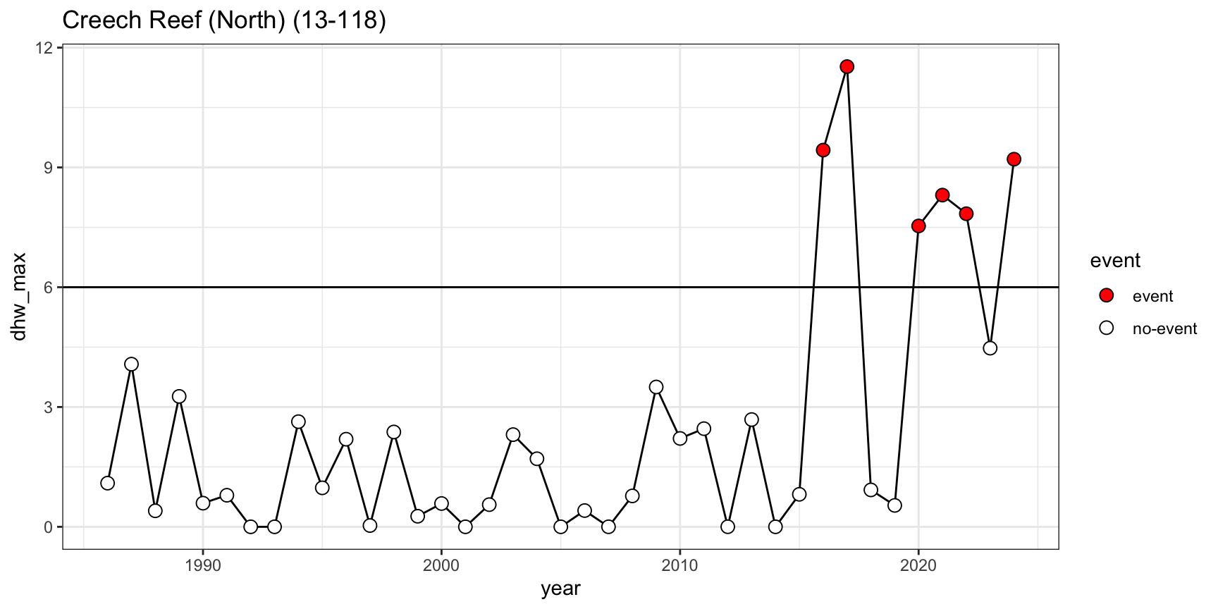
5) Emerging heat stress on previously unimpacted reefs
For reefs that have been impacted in 2024 event (>4 DHW), how long has the recovery time since they last experienced >4DHW conditions?
- The majority of reefs that were impacted by the 2024 event by at least 4DHW have experienced a similar conditions (>4DHW) either in the 2020-2022 events (35.1% of reefs), or in the 2016-2017 events (32.7%).
- A subset of reefs in the southern GBR that were impacted in the 2024 have previously been considered a “refuge” from thermal stress, and have experienced thermal stress (>4DHW) for the first time in over thirty years (31.2% of total).
- In the southern GBR, 111 reefs (3% of total) that were impacted by >4DHW conditions in the 2024 event have no record of >4DHW conditions in the entire record (1986-2024).
# Get all reefs in 2024 that are >4 DHW
dhw_reefs_2024 <- gbr_shape_dhw |>
as.data.frame() |> # 3,716 reef_id
dplyr::select(-geometry, -id, -gbr_name) |>
pivot_longer(-c(reef_id), names_to="year", values_to="dhw_max") |>
mutate(year = as.numeric(substr(year, nchar(year)-3, nchar(year)))) |>
filter(!dhw_max < 4) |> # drop reefs with less than 4 DHW
filter(year==2024) #
dhw_reefs_any <- gbr_shape_dhw |> # top DHW that wasn't 2024 and is > 4DHW
as.data.frame() |> # 3,716 reef_id
dplyr::select(-geometry, -id, -gbr_name) |>
pivot_longer(-c(reef_id), names_to="year", values_to="dhw_max") |>
mutate(year = as.numeric(substr(year, nchar(year)-3, nchar(year)))) |>
filter(!dhw_max < 4) |> # drop reefs with less than 4 DHW
filter(!year == 2024) |>
group_by(reef_id) |>
top_n(n=1) |> # keep top year
rename(warmest_year=year, warmest_dhw_max=dhw_max)
dhw_reefs_2024_comparison <- left_join(dhw_reefs_2024, dhw_reefs_any, by="reef_id") |>
mutate(time_since = year - warmest_year) |>
mutate(time_since = ifelse(is.na(time_since), 38, time_since)) |>
mutate(time_since=as.numeric(time_since)) |>
mutate(bins=cut(time_since, c(0, 5, 10, 20, 30, 40),
labels=c("1-5yrs", "5-10yrs", "10-20yrs",
"20-30yrs", "30-40yrs")))
#dhw_reefs_2024_comparison[!complete.cases(dhw_reefs_2024_comparison), ]
dhw_reefs_2024_comparison_count <- dhw_reefs_2024_comparison %>%
group_by(bins) %>%
summarise(count = n()) |>
mutate(proportion= (count/sum(count)*100))
record_a <- ggplot() + theme_bw() + ylab("Proportion of reefs\n") +
geom_col(data=dhw_reefs_2024_comparison_count, aes(x=bins, y=proportion, fill=bins),
color="black", show.legend=FALSE) + ylim(0,60) +
geom_text(data=dhw_reefs_2024_comparison_count, aes(x=bins, y=proportion+2,
label=c("1-5yrs", "5-10yrs", "10-20yrs",
"20-30yrs", "30-40yrs")), size=3) +
scale_fill_manual(values=rev(c("#b70000","#74b9e6", "#89d3db", "#cdd888", "#e8d277")))
# list reefs
no_record_reefs <- dhw_reefs_2024_comparison |> filter(bins == ">30 yrs") |> pluck("reef_id")
# map spatial patterns
no_record_reefs_spatial <- gbr_shape_dhw |>
left_join(dhw_reefs_2024_comparison |>
select(reef_id, bins)) |>
na.omit() # remove unimpacted reefs
record_b <- no_record_plot <- ggplot() + theme_bw() + facet_wrap(~bins) +
geom_sf(data=ausmap, fill="olivedrab4", alpha=0.2) +
geom_sf(data=no_record_reefs_spatial, aes(fill=bins), shape=21, stroke=0.1) +
theme(axis.text.x = element_text(angle = 45, hjust = 1)) +
scale_fill_manual(values=rev(c("#b70000","#74b9e6", "#89d3db", "#cdd888", "#e8d277")))
record_a|record_b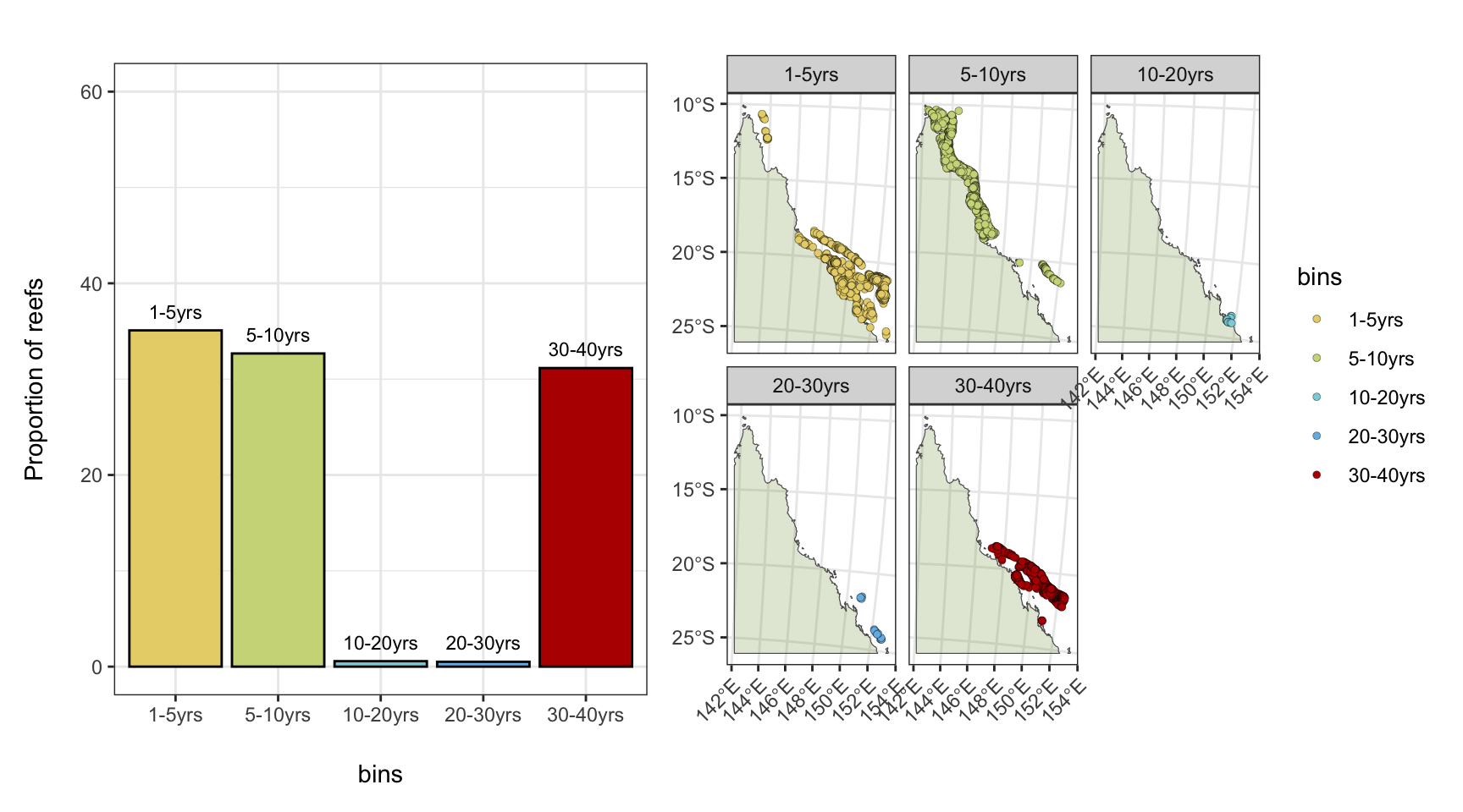
6) Trajectories of DHW on the GBR
A (very) simple analysis of the time-series for the 3,716 reefs on the GBR indicates increasing trajectories of DHW across the 38 year time period (note: preliminary, a more detailed analysis is required to quantify these trends):
library(tidyverse)
library(sf)
library(ggplot2)
library(plotly)
# https://zenodo.org/records/5146061/preview/ymbozec/REEFMOD.6.4_GBR_HINDCAST_ANALYSES-v1.0.0.zip
# make a new zones for whole id
id_zones <- read.csv("/Users/rof011/GBR-coral-bleaching/data/gbr_zones.csv") |>
mutate(id=str_replace(label_id, "[a-zA-Z]$", "")) |>
dplyr::select(-label_id, -X) |>
distinct()
gbr_shape_dhw_centroid <- gbr_shape_dhw |>
st_centroid() |>
st_coordinates() |>
as.data.frame() |>
rename(lon=1, lat=2)
gbr_shape_dhw_zones_long <- gbr_shape_dhw %>%
as.data.frame() %>%
dplyr::select(-geometry) %>%
cbind(., gbr_shape_dhw_centroid) %>%
pivot_longer(cols = starts_with("dhw_max_"), names_to = "year", values_to = "dhw_max") %>%
mutate(year = str_replace(year, "dhw_max_", "")) %>%
left_join(id_zones, by="id") |>
mutate(reef_id = paste0(as.character(gbr_name), " (", id,")")) |>
group_by(gbr_name) |>
mutate(max=max(dhw_max))
p1 <- ggplot() + geom_smooth(data = gbr_shape_dhw_zones_long |> na.omit() |> droplevels(),
aes(x=year, y=dhw_max, group=reef_id, text=reef_id), show.legend = FALSE,
se = FALSE, method = "gam", formula = y ~ s(x, bs = "cr", k = 10))
max_spline <- ggplot_build(p1)$data |>
as.data.frame() |>
dplyr::select(text, y) |>
rename(reef_id=text) |>
group_by(reef_id) |>
slice(which.max(y)) |>
rename(max=y)
plot_data <- ggplot_build(p1)$data |>
as.data.frame() |>
dplyr::select(text, x, y) |>
rename(reef_id=text, year=x, dhw_max=y) |>
left_join(max_spline, by="reef_id")
# Your original ggplot code
p2 <- ggplot() + theme_bw() +
geom_smooth(data=plot_data |> na.omit() |> droplevels(),
aes(x=year, y=dhw_max, group=reef_id, color=max), #color="darkgrey",
se = FALSE, linewidth=0.09, method = "gam",
formula = y ~ s(x, bs = "cr", k = 10), show.legend = FALSE) +
theme(axis.text.x = element_text(angle = 90, vjust = 0.5, hjust=1)) +
scale_color_distiller(palette = "Reds", direction = 1, limits=c(1,9))
# Convert to ggplotly
ggplotly(p2, tooltip = c("reef_id", "year", "dhw_max"))