Site selection

---

Comparisons of various approaches to determine optimal placement of restoration areas given an underlying habitat shp file using Lizard Island example from Allen Coral Atlas.

---

Import habitats

1. import shp files, filter and remove polygons less than target plot hectare size (1ha).

Red inset box = subset map used below (note - spatial data in projected coordinate system 20353)

library(tidyverse)
library(sf)
library(future.apply)
library(tictoc)
library(lwgeom)
library(tmap)

set.seed(123)


# Import reef polygons, create union (or returns multiple intersections 
geomorphic_seeding <- st_read("/Users/rof011/spatialtools/apps/remove-zones/www/geomorphic.geojson", quiet=TRUE) %>% 
  mutate(area=as.numeric(st_area(.))) |> 
  st_transform(20353) |> 
  filter(area > 10000) |> 
  mutate(n=round(as.numeric(area)/1000)) |> 
  st_transform(4326) |> 
  st_crop(st_bbox(c(xmin = 145.42, xmax = 145.48, ymin = -14.72, ymax = -14.64))) |> 
  st_transform(20353) 

geomorphic_seeding_filtered <-  geomorphic_seeding %>%
  filter(class %in% c("Outer Reef Flat", "Reef Slope", "Back Reef Slope"))
 
inset <- st_bbox(c(xmin = 145.44, xmax = 145.455, ymin = -14.697, ymax = -14.692)) |> 
  st_bbox()

inset_sf <- inset |> st_as_sfc() |> st_set_crs(4326)

habitat_pal <- c("Plateau" = "cornsilk2", "Back Reef Slope" = "darkcyan",
  "Reef Slope" = "darkseagreen4", "Sheltered Reef Slope" = "darkslategrey",
  "Inner Reef Flat" = "darkgoldenrod4", "Outer Reef Flat" = "darkgoldenrod2",
  "Reef Crest" = "coral3",  "Shallow Lagoon" = "turquoise3",
  "Deep Lagoon" = "turquoise4")


habitat_pal_filtered <- c("Back Reef Slope" = "darkcyan",
  "Reef Slope" = "darkseagreen4", "Sheltered Reef Slope" = "darkslategrey",
  "Outer Reef Flat" = "darkgoldenrod2")




tmap_mode("plot")
tm_basemap("Esri.WorldImagery", alpha=0.6) +
tm_shape(geomorphic_seeding) +
  tm_polygons(fill="class",
              lwd=0,
              fill_alpha=0.7,
              fill.scale=tm_scale_categorical(values=habitat_pal)) +
tm_shape(inset_sf) +
  tm_polygons(fill=NA,
             col="red",
             lwd=2)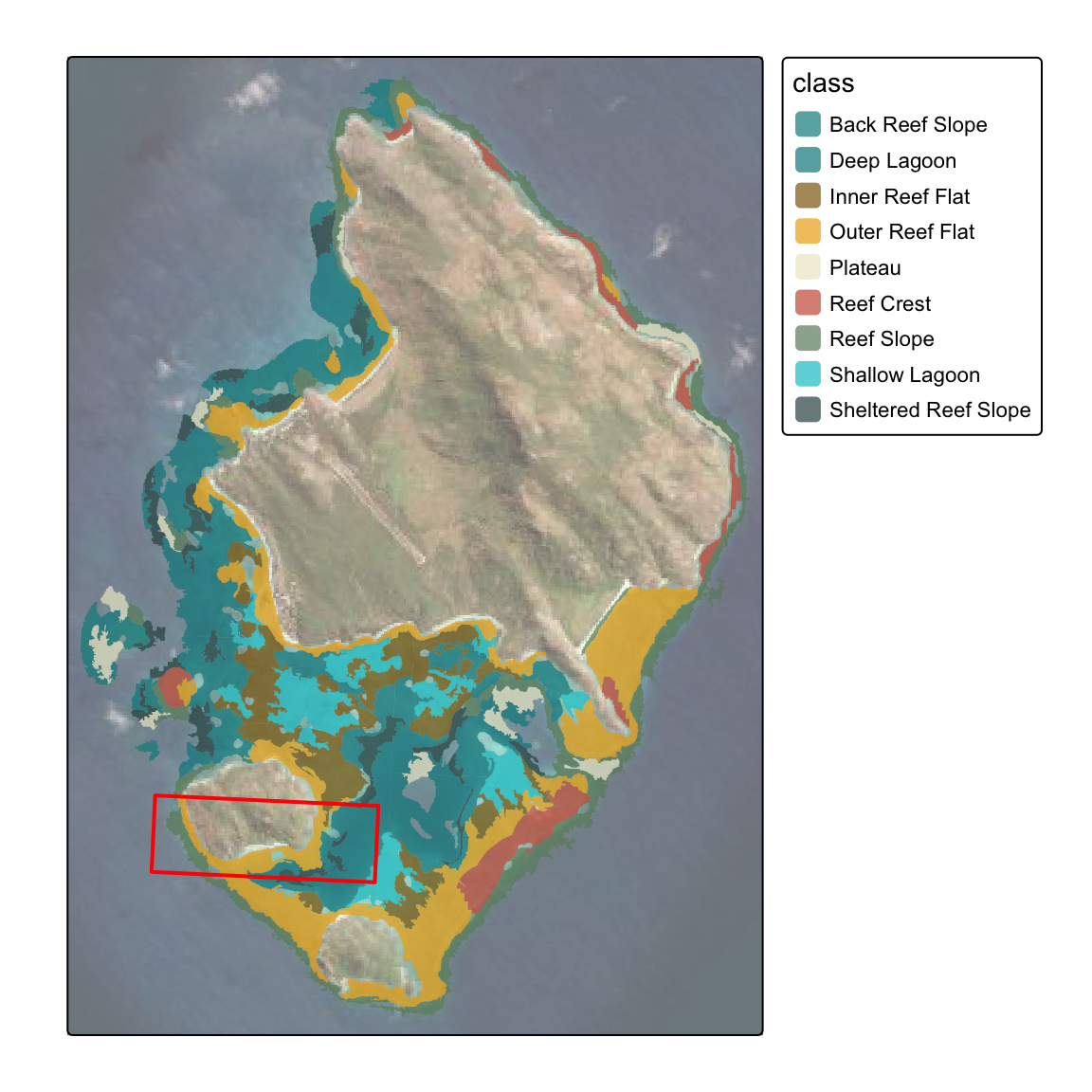

---

1) grid polygons

Determine optimum plot 1ha locations using a regular parallel grid (100m x 100m).

• for simplicity habitat was filtered to restrict polygons to selected four habitat types (“Outer Reef Flat”, “Reef Slope”, “Back Reef Slope”, “Sheltered Reef Slope”)
• white polygons in map below represent 100m x 100m grid cells with 100% coverage of underlying habitat types
• note: code throughout retains 100% coverage in polygons, but set threshold as needed.

geomorphic_seeding_union <- geomorphic_seeding %>%
  filter(class %in% c("Outer Reef Flat", "Reef Slope", "Back Reef Slope", "Sheltered Reef Slope")) %>%
  st_snap_to_grid(size = 0.01) %>%
  st_make_valid() %>% 
  st_buffer(dist=0.1) %>%
  group_by() %>% 
  summarise(area = sum(area)) %>% 
  ungroup() 

geomorphic_seeding_buffered <- st_buffer(geomorphic_seeding_union, dist = 100)
bbox <- st_bbox(geomorphic_seeding_buffered)
grid <- st_make_grid(bbox, cellsize = c(100, 100), square = TRUE)
grid_sf <- st_sf(geometry = grid)

contains_properly <- st_contains_properly(geomorphic_seeding_union, grid_sf)
indices <- unlist(contains_properly)
indices_numeric <- as.numeric(indices)
grid_sf_whole <- grid_sf[indices_numeric, ]

# Visualization with tmap
tm_basemap("Esri.WorldImagery") +
tm_shape(geomorphic_seeding_filtered, bbox=inset) +
  tm_polygons(fill = "class", 
              fill.legend = tm_legend(title="Habitat", position = tm_pos_out("right", "center")),
              fill.scale=tm_scale_categorical(values=habitat_pal_filtered), 
              lwd = 0.2, col="black", fill_alpha = 1) +
  tm_shape(grid_sf, bbox = inset, crs = 20353) +
  tm_polygons(fill = NA, col = "darkred", lwd = 0.5) +
  tm_shape(grid_sf_whole, bbox = inset, crs = 20353) +
  tm_polygons(fill = NA, col = "white", lwd = 1)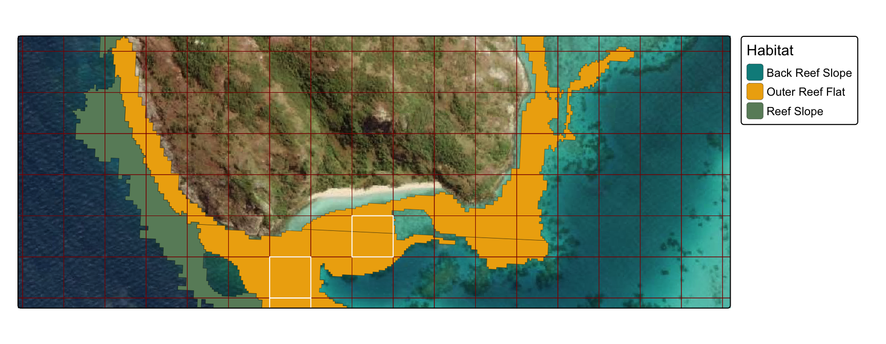 

to iterate, use lapply to shift the grid by 10m increments in lon and lat (or finer resolution):

library(sf)
library(dplyr)
library(tmap)

# Ensure CRS is set to 20353
crs_value <- 20353

# Define the steps for shifting the grid
step_size <- 10
shifts <- seq(0, 90, by = step_size)  # 10m steps up to 90m

bbox <- st_bbox(geomorphic_seeding_union)

# Function to shift grid and filter based on st_contains_properly
generate_shifted_grid <- function(shift_x, shift_y) {
  # Shift the bounding box
  shifted_bbox <- bbox
  shifted_bbox['xmin'] <- bbox['xmin'] + shift_x
  shifted_bbox['xmax'] <- bbox['xmax'] + shift_x
  shifted_bbox['ymin'] <- bbox['ymin'] + shift_y
  shifted_bbox['ymax'] <- bbox['ymax'] + shift_y
  
  # Ensure that the shifted_bbox values are valid
  if (any(is.na(shifted_bbox))) {
    stop("Shifted bounding box contains NA values, check your shifts.")
  }
  
  # Generate the grid and set the CRS
  grid <- st_make_grid(shifted_bbox, cellsize = c(100, 100), square = TRUE)
  grid_sf <- st_sf(geometry = grid, crs = crs_value)
  
  # Check if grid cells are fully within the geomorphic_seeding_union
  contains_properly <- st_contains_properly(geomorphic_seeding_union, grid_sf)
  indices <- unlist(contains_properly)
  
  # Add a color column based on whether the grid cells are fully contained
  grid_sf <- grid_sf %>%
    mutate(color = ifelse(row_number() %in% indices, "complete", "partial"))
  
  return(grid_sf)
}

# Apply the function over all combinations of shifts in x and y directions
grids_list <- lapply(shifts, function(x_shift) {
  lapply(shifts, function(y_shift) {
    generate_shifted_grid(x_shift, y_shift)
  })
})


# Flatten the nested list of sf objects into a single list
flattened_list <- do.call(c, grids_list)

# Combine all sf objects into a single sf object
grids_list <- do.call(rbind, flattened_list)

gridplots <- tm_basemap("Esri.WorldImagery") +
tm_shape(geomorphic_seeding_filtered, bbox=inset) +
  tm_polygons(fill = "class", 
              fill.legend = tm_legend(title="Habitat",  bg.color="lightgrey", position = tm_pos_out("right", "center")),
              fill.scale=tm_scale_categorical(values=habitat_pal_filtered), 
              lwd = 0.2, col="black", fill_alpha = 1) + 
  tm_shape(grids_list, bbox = inset, crs = 20353) +
    tm_polygons(fill = NA, col = "color", lwd = "color", 
                col.legend = tm_legend(title="Plots", bg.color="lightgrey", position = tm_pos_out("right", "center")),
                col.scale=tm_scale_categorical(values=c("white", "darkred")), 
                lwd.scale=tm_scale_categorical(values=c(1, 0.1)),
                lwd.legend=tm_legend_hide()
                ) +
  tm_title("1) Gridded plots")
  
gridplots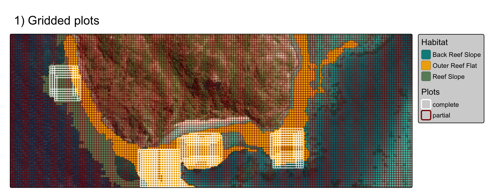

---

2) parallel random polygons

Determine optimum plot 1ha locations using polygons with randomly seeded centroids, keep polygons that are 100% overlap with habitat type.

The number of seed points (centroids for polygons) is determined by the area of each polygon (i.e. larger polygons = more points)

set.seed(101)

#remotes::install_github("r-tmap/tmap.deckgl")

# lapply sampling process
seeded_points <- st_sf(do.call(rbind, lapply(seq_len(nrow(geomorphic_seeding_filtered)), function(i) {
  polygon <- geomorphic_seeding_filtered[i, ]
  points <- st_sample(polygon, size = polygon$n, type = "random")
  st_sf(class = polygon$class, geometry = points)
}))) |> st_transform(20353)


tm_basemap("Esri.WorldImagery") +
tm_shape(geomorphic_seeding_filtered) +
  tm_polygons(fill = "class", 
              fill.legend = tm_legend(title="Habitat", position = tm_pos_out("right", "center")),
              fill.scale=tm_scale_categorical(values=habitat_pal_filtered), 
              lwd = 0.2, col="black", fill_alpha = 1) +
tm_shape(seeded_points) +
  tm_dots(size=0.05, 
          fill="white",
          fill_alpha=0.5) +
tm_shape(inset_sf) +
  tm_polygons(fill=NA,
             col="red",
             lwd=2) +
tm_title("Random seed centroids for polygons")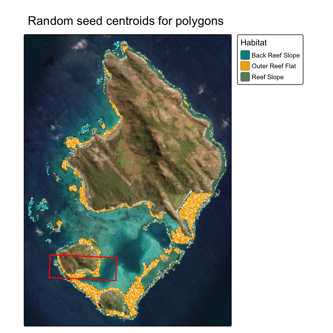

Generate 100 x 100m polygons around each point:

# Define the width and length of the rectangle
width <- 100  # Example width (in the same units as your CRS)
length <- 100  # Example length (in the same units as your CRS)

# Use lapply to create the buffered polygons
buffered_polygons <- lapply(seq_len(nrow(seeded_points)), function(i) {
  
  # Extract the coordinates of the current point
  x <- sf::st_coordinates(seeded_points)[i, 1]
  y <- sf::st_coordinates(seeded_points)[i, 2]
  
  # Set parameters for the rectangle around the point
  x_min <- x - (width / 2)
  x_max <- x + (width / 2)
  y_min <- y - (length / 2)
  y_max <- y + (length / 2)
  
  # Create the rectangular polygon
  polygon <- sf::st_polygon(list(rbind(
    c(x_min, y_min), 
    c(x_min, y_max), 
    c(x_max, y_max), 
    c(x_max, y_min), 
    c(x_min, y_min)
  )))
  
  return(polygon)
})

# Combine the results into a single sf object
buffered_polygons_sf <- sf::st_sfc(buffered_polygons, crs = sf::st_crs(seeded_points)) |> st_as_sf()


tm_basemap("Esri.WorldImagery") +
tm_shape(geomorphic_seeding_filtered, bbox=inset) +
  tm_polygons(fill = "class", 
              fill.legend = tm_legend(title="Habitat", position = tm_pos_out("right", "center")),
              fill.scale=tm_scale_categorical(values=habitat_pal_filtered), 
              lwd = 0.2, col="black", fill_alpha = 1) +
tm_shape(buffered_polygons_sf,
         bbox=inset,
         crs=20353) +
  tm_polygons(fill=NA,
              col="white",
              lwd=0.8)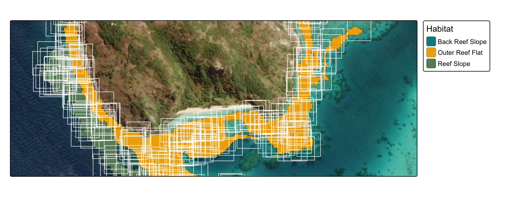 

Make a function to apply plots across points using lapply and retain only polygons with 100% overlap with reef habitats as with gridded approach and time using tictoc:

library(tictoc)

tic()
# lapply sampling process
seeded_points <- st_sf(do.call(rbind, lapply(seq_len(nrow(geomorphic_seeding_filtered)), function(i) {
  polygon <- geomorphic_seeding_filtered[i, ]
  points <- st_sample(polygon, size = polygon$n, type = "random")
  st_sf(class = polygon$class, geometry = points)
}))) |> st_transform(20353)


# Define the width and length of the rectangle
width <- 100  
length <- 100 

# Use lapply to create the buffered polygons
buffered_polygons_filtered <- lapply(seq_len(nrow(seeded_points)), function(i) {
  
  # Extract the coordinates of the current point
  x <- sf::st_coordinates(seeded_points)[i, 1]
  y <- sf::st_coordinates(seeded_points)[i, 2]
  
  # Set parameters for the rectangle around the point
  x_min <- x - (width / 2)
  x_max <- x + (width / 2)
  y_min <- y - (length / 2)
  y_max <- y + (length / 2)
  
  # Create the rectangular polygon
  polygon <- sf::st_polygon(list(rbind(
    c(x_min, y_min), 
    c(x_min, y_max), 
    c(x_max, y_max), 
    c(x_max, y_min), 
    c(x_min, y_min)
  )))
  
  return(polygon)
})

# Combine the results into a single sf object
buffered_polygons_filtered_sf <- sf::st_sfc(buffered_polygons_filtered, crs = sf::st_crs(seeded_points)) |> st_as_sf()


# Intersect the plots with the reef polygons, calculate overlap
intersections_filtered <- st_intersection(buffered_polygons_filtered_sf, st_union(geomorphic_seeding_filtered)) %>%
  mutate(intersection_area = st_area(.)) %>%
  mutate(percentage_overlap = (as.numeric(intersection_area)/10000) * 100) |> 
  mutate(overlap=ifelse(percentage_overlap==100, "complete", "partial")) 

toc()

## 4.724 sec elapsed

tmap_mode("plot")
polyplots <- tm_basemap("Esri.WorldImagery") +
tm_shape(geomorphic_seeding_filtered, bbox=inset) +
  tm_polygons(fill = "class", 
              fill.legend = tm_legend(title="Habitat", bg.color="lightgrey", position = tm_pos_out("right", "center")),
              fill.scale=tm_scale_categorical(values=habitat_pal_filtered), 
              lwd = 0.2, col="black", fill_alpha = 1) +
tm_shape(intersections_filtered, 
         bbox=inset) +
  tm_polygons(fill = NA, col = "overlap", lwd = "overlap", 
                col.legend = tm_legend(title="Plots", bg.color="lightgrey", position = tm_pos_out("right", "center")),
                col.scale=tm_scale_categorical(values=c("white", "darkred")), 
                lwd.scale=tm_scale_categorical(values=c(1, 0.2)),
                lwd.legend=tm_legend_hide()
                ) +
tm_title("2) Random parallel polygons", size=1)

polyplots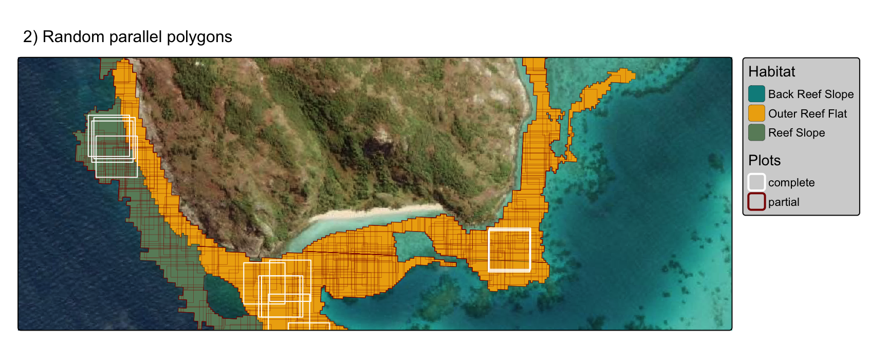

Use future.lapply to speed things up with larger datasets (note: multisession below, use multicoreon base R to obtain optimal results)

options(future.rng.onMisuse = "ignore")
library(future.apply)

tic()

# Set up parallel processing plan
plan(multisession, workers = availableCores())

# Parallel lapply sampling process using future_lapply
seeded_points_list <- future_lapply(future.seed=NULL, seq_len(nrow(geomorphic_seeding)), function(i) {
  polygon <- geomorphic_seeding[i, ]
  points <- st_sample(polygon, size = polygon$n, type = "random")
  st_sf(class = polygon$class, geometry = points)
})

# Combine the list into a single sf object
seeded_points <- do.call(rbind, seeded_points_list) |> st_sf() |> st_transform(20353)

# Define the width and length of the rectangle
width <- 100  # Example width (in the same units as your CRS)
length <- 100  # Example length (in the same units as your CRS)

# Use future_lapply to create the buffered polygons
buffered_polygons_list <- future_lapply(seq_len(nrow(seeded_points)), function(i) {
  
  # Extract the coordinates of the current point
  x <- sf::st_coordinates(seeded_points)[i, 1]
  y <- sf::st_coordinates(seeded_points)[i, 2]
  
  # Set parameters for the rectangle around the point
  x_min <- x - (width / 2)
  x_max <- x + (width / 2)
  y_min <- y - (length / 2)
  y_max <- y + (length / 2)
  
  # Create the rectangular polygon
  polygon <- sf::st_polygon(list(rbind(
    c(x_min, y_min), 
    c(x_min, y_max), 
    c(x_max, y_max), 
    c(x_max, y_min), 
    c(x_min, y_min)
  )))
  
  return(polygon)
})

# Combine the results into a single sf object
buffered_polygons_sf <- sf::st_sfc(buffered_polygons_list, crs = sf::st_crs(seeded_points)) |> st_as_sf()

# Intersect the plots with the reef polygons, calculate overlap
intersections <- st_intersection(buffered_polygons_sf, st_union(geomorphic_seeding)) %>%
  mutate(intersection_area = st_area(.)) %>%
  mutate(percentage_overlap = (as.numeric(intersection_area) / 10000) * 100)

# Reset the plan to sequential processing after completion (optional)
plan(sequential)

toc()

---

3) rotated random polygons

• Determine optimum plot 1ha locations using polygons with randomly seeded centroids

• rotate polygons by a random 5° compass bearing between 0-355°.

• retain polygons that are 100% overlap with habitat type.

• use future.lapply to multisession and time using tictoc

library(future.apply)
library(sf)
library(spatialEco)

tic()

# Set up parallel processing plan
plan(multisession, workers = availableCores())

# Use future_lapply to create the buffered polygons with random rotations
buffered_polygons_list_rotated <- future_lapply(seq_len(nrow(seeded_points)), function(i) {
  
  # Extract the coordinates of the current point
  x <- sf::st_coordinates(seeded_points)[i, 1]
  y <- sf::st_coordinates(seeded_points)[i, 2]
  
  # Set parameters for the rectangle around the point
  x_min <- x - (width / 2)
  x_max <- x + (width / 2)
  y_min <- y - (length / 2)
  y_max <- y + (length / 2)
  
  # Create the rectangular polygon
  polygon <- sf::st_polygon(list(rbind(
    c(x_min, y_min), 
    c(x_min, y_max), 
    c(x_max, y_max), 
    c(x_max, y_min), 
    c(x_min, y_min)
  )))
  
  # Convert to sf object for rotation
  polygon_sf <- st_sf(geometry = st_sfc(polygon, crs = st_crs(seeded_points)))
  
  # Select a random rotation angle from the sequence
  angle <- sample(seq(0, 355, 5), 1)
  
  # Rotate the polygon by the random angle using spatialEco::rotate.polygon
  rotated_polygon <- spatialEco::rotate.polygon(polygon_sf, angle = angle, anchor = "center")  |> mutate(id=i)
  # Extract the geometry from the rotated sf object
  return(rotated_polygon)
})

buffered_polygons_rotated <- do.call(rbind,buffered_polygons_list_rotated) |> st_set_crs(20353)

buffered_polygons_rotated_intersect <- st_intersection(buffered_polygons_rotated, st_union(geomorphic_seeding_filtered)) %>% 
                                mutate(intersection_area = st_area(.)) |> as.data.frame() |> select(-geometry)

intersections_rotated <- buffered_polygons_rotated |> 
  left_join(buffered_polygons_rotated_intersect, by="id") |> 
  mutate(percentage_overlap = (as.numeric(intersection_area) / 10000) * 100) |> 
  mutate(overlap=ifelse(percentage_overlap>98, "complete", "partial")) 



# Reset the plan to sequential processing after completion (optional)
plan(sequential)

toc()

## 9.133 sec elapsed

inset <- st_bbox(c(xmin = 145.44, xmax = 145.455, ymin = -14.697, ymax = -14.692)) |> 
  st_bbox()


tmap_mode("plot")
rotatedplots <- tm_basemap("Esri.WorldImagery") +
tm_shape(geomorphic_seeding_filtered, bbox=inset) +
  tm_polygons(fill = "class", 
              fill.legend = tm_legend(title="Habitat",  bg.color="lightgrey", position = tm_pos_out("right", "center")),
              fill.scale=tm_scale_categorical(values=habitat_pal_filtered), 
              lwd = 0.2, col="black", fill_alpha = 1) +
tm_shape(intersections_rotated,
         bbox=inset) +
  tm_polygons(fill = NA, col = "overlap", lwd = "overlap", 
                col.legend = tm_legend(title="Plots", bg.color="lightgrey", position = tm_pos_out("right", "center")),
                col.scale=tm_scale_categorical(values=c("white", "darkred")), 
                lwd.scale=tm_scale_categorical(values=c(1, 0.2)),
                lwd.legend=tm_legend_hide()
                ) +
tm_title("3) Rotated random polygons", size=1)

rotatedplots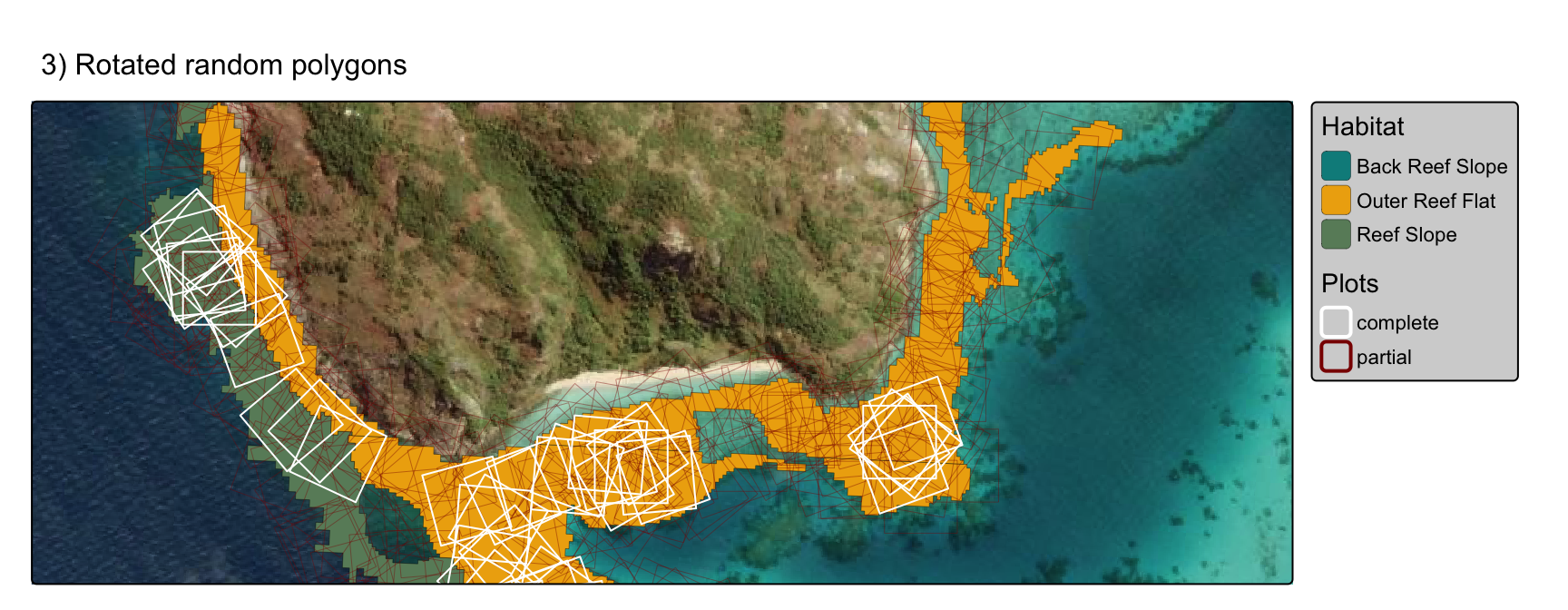

---

Outputs

Summary points below:

i) rotating polygons doesn’t increase total plot numbers

Broadly similar outputs for percent overlap between the paralell and rotated plot aproaches:

combined <- rbind(intersections_filtered |> mutate(type="Parallel plots") |> as.data.frame() |> select(intersection_area, type),
                  buffered_polygons_rotated_intersect |> mutate(type="Rotated plots") |> as.data.frame() |> select(intersection_area, type)
                )  
  
combined <- combined |> mutate(percentage_overlap=as.numeric(intersection_area)/10000*100)

combined_data <- as.data.frame(combined)
hist_data <- ggplot_build(ggplot(combined_data) + geom_histogram(aes(x = percentage_overlap, fill = type)))$data[[1]]
scale_factor <- max(hist_data$count) / max(hist_data$density)

ggplot() + 
  theme_bw() + 
  facet_wrap(~type) +
  stat_density(data = combined_data, aes(x = percentage_overlap, y = ..density.. * scale_factor, col = type), 
                 alpha = 0.2, linewidth = 0.5, show.legend=FALSE, fill=NA) +
  geom_histogram(data = combined_data, aes(x = percentage_overlap, y = ..count.., fill = type), 
                 alpha = 0.2, color = "black", linewidth = 0.2, show.legend=FALSE) +
 
  scale_y_continuous(
    name = "Count",
    sec.axis = sec_axis(~ . / scale_factor, name = "Density")
  ) + 
  scale_fill_manual(values=c("turquoise4", "coral4")) +
  scale_color_manual(values=c("turquoise4", "coral4"))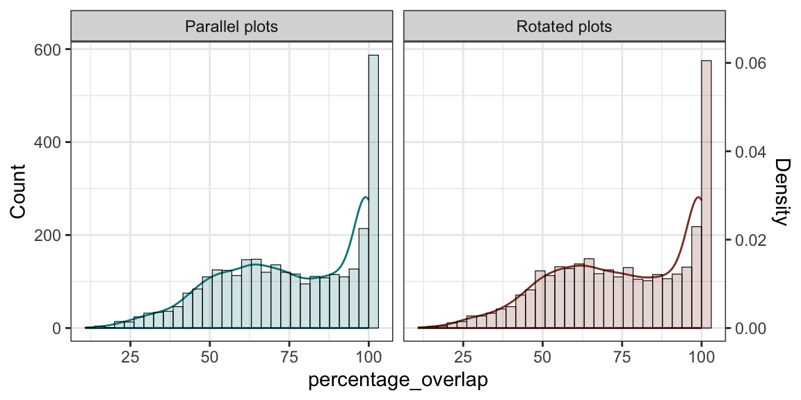

ii) rotating plots improves fit in narrow polygons

The rotated plot method appears to improve fit in narrow irregular polygons over both the regular gridded plot and random plot approaches:

tmap_arrange(gridplots, polyplots, rotatedplots, ncol=1)

iii) efficiency over large areas

To be explored: sf is very slow for large computations. Opt for shapely or geopandas and optimise:

from shapely.geometry import Polygon
from shapely.affinity import rotate

import geopandas as gpd
from shapely.affinity import rotate