About D^₃HW

D^₃W is a data visualisation of the annual heatstress (DHW) for each reef on the Great Barrier Reef. Each row represents a reef (4306 reefs in total), each column represents the amount of heat stress experienced (between 1981 and 2025). The colors represent the maximum heat stress in a given year: in simple terms,

normal• coral bleaching • strong coral bleaching • likely catastrophic bleaching

D^₃HW was created using the D3 library in javascript - hence the term D^₃ egree Heating Weeks.

Degree Heating Weeks explained

Corals are sensitive to warmer temperatures: at around one degree Celsius (1 °C) above the highest annual mean temperature corals exceed their “bleaching threshold”. Degree Heating Weeks (DHW) are a useful metric of cumulative heatstress (i.e. how many times in the last twelve weeks has the temperature reached or exceeded the bleaching threshold?). From NOAA:

“By the time the accumulated heat stress (the DHW) reaches 4 °C-weeks, you can expect to see coral bleaching reef-wide, especially in more sensitive coral species. By the time the DHW value reaches 8 °C-weeks or higher, you are likely to see reef-wide coral bleaching with mortality of heat-sensitive corals”

Why D^₃HW?

Sea Surface Temperature (SST) data is widely accessible from various satellites, but is often hard to visualise. Questions like “how bad is this year’s bleaching compared to last year?”, and “How many reefs are affected by bleaching?” are difficult to map due to the size of the Great Barrier Reef, and time-series charts often mask the impacts on individual reefs.

D^₃HW aims to i) simplify long-term trends in temperature and climate change on the Great Barrier Reef, and ii) highlight that intense heatwaves on the Great Barrier Reef are a recent phenomena, and not a “normal” state.

GBR D^₃HW

The impact of coral bleaching on the Great Barrier Reef (GBR) takes time to assess through surveys, yet the link between DHW and both coral bleaching and coral mortality are well documented on the Great Barrier Reef.

Unlike the recent bushfires where the impacts of climate-change driven heatwaves are clearly visible, the recent mass coral bleaching events on the Great Barrier Reef have largely gone by unreported as they unfolded - despite satellite data being readily available in near real-time.

As one journalist put to me recently: “if a bleaching event is underway on the GBR and no reporting on the temperature data, how can anyone know the size and scale that these events are actually occuring?”

D^₃HW aims to make satellite data more accessible to non-scientific audiences, allowing comparisons between current heat-stress levels with previous events, and facilitating tracking of coral bleaching events as they occur in realtime.

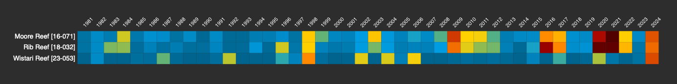
Reef-level tracking of annual DHW

D^₃HW aims to make it easier to visualise time-series of Degree Heating Weeks for any reef on the GBR. For example, comparing Moore Reef (Cairns), Rib Reef (Townsville), and Wistari Reef (southern GBR) highlights how Wistari in the south avoided heatstress for nearly a decade prior to the 2024 mass bleaching event, while Moore Reef and Rib Reef further north have been impacted repeatedly by heatwaves in 2016, 2017, 2020, 2021, 2022, and 2024.

Mass coral bleaching and the GBR

The Great Barrier Reef is undergoing rapid warming in the past three decades. A total of nine coral bleaching events have been recorded in 1998, 2002, 2016, 2017, 2018, 2020, 2022, 2024, and 2025. These events have resulted in mass mortality of corals, impacting coral population structures, transforming assemblages, delaying recovery and restructuring entire ecosytems.

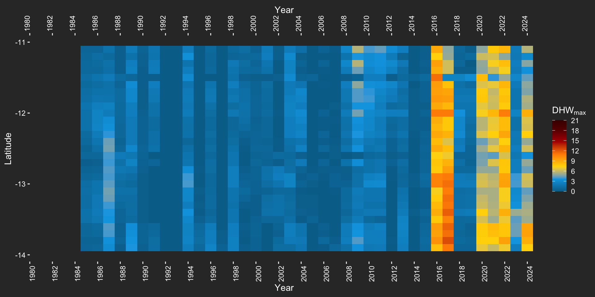
Long-term timeseries data helps prevent normalising the current state by providing historical context. For example, here is a timeseries for 560 reefs in the northern GBR spanning Lama Lama Sea Country to the Wuthathi sea country:

library(tidyverse)

library(ggplot2)

GBR_DHW_CRW <- read.csv("/Users/rof011/dhw3/data/CRW_DHWmax.csv") |> 

  pivot_longer(

    cols = starts_with("X"),

    names_to = "year",

    values_to = "dhw"

  ) %>%

  mutate(

    year = as.numeric(str_remove(year, "^X"))

  ) |> filter(lat < -11) |> filter(lat > -14)

dhw_numeric_breaks <- c(0, 3, 6, 9, 12, 15, 18, 21)  # Adjust numeric breaks

dhw_colour_breaks <- c("#006f99", "#00A6E5", "#FFD700", "#FF8C00", "#B20000", "#660000", "#3D0000")

ggplot() + theme_bw() +

  geom_tile(data = GBR_DHW_CRW, aes(x = year, y = lat, fill = dhw), linewidth = 0) +

  scale_fill_gradientn(

    limits = c(0, 21),

    name = expression(DHW[max]),

    na.value = "transparent",

    breaks = dhw_numeric_breaks,

    labels = dhw_numeric_breaks,

    colours = dhw_colour_breaks,

    values = scales::rescale(dhw_numeric_breaks, from = c(0, 20))

  ) +

  xlab("Year") + ylab("Latitude") +

  # scale_y_continuous(

  #   expand = c(0, 0),

  #   limits = c(-11,-13),

  #   breaks = seq(-11,-13, length.out=5), 

  #   labels = seq(-11,-13, length.out=5)

  # ) +

   scale_x_continuous(

    expand = c(0, 0),

    limits = c(1980, 2025),

    breaks = seq(1980, 2025, 2),

    sec.axis = dup_axis(name = "Year")

  ) +

  theme(

    # Backgrounds

    plot.background = element_rect(fill = "#333", color = NA),

    panel.background = element_rect(fill = "#333", color = NA),

    panel.grid = element_blank(),

    

    # Axes

    axis.title = element_text(color = "white"),

    axis.text = element_text(color = "white"),

    axis.text.x = element_text(angle = 90, hjust = 1, color = "white"),

    axis.text.y = element_text(color = "white", hjust=-0.2),

    axis.ticks = element_line(color = "white"),

    

    # Secondary axis text and title

    axis.title.x.top = element_text(color = "white"),

    axis.text.x.top = element_text(color = "white"),

    

    # Legend

    legend.background = element_rect(fill = "#333", color = NA),

    legend.key = element_rect(fill = "#333", color = NA),

    legend.text = element_text(color = "white"),

    legend.title = element_text(color = "white"),

    

    # Titles

    plot.title = element_text(color = "white"),

    plot.subtitle = element_text(color = "white"),

    plot.caption = element_text(color = "white")

  )

Datasets used in D^₃HW:

DHW uses

Contact

DHW uses